Calibration of a Piezoelectric Accelerometer by Comparison to a Reference Transducer
Introduction
Today’s modern technology is full of sensors. Sensing temperature, motion, force, humidity, sound, electricity, radiation – basically every imaginable physical quantity – necessary to measure and understand our environment. This is usually done with so-called transducers (sometimes abbreviated as Xducers) which convert the measured physical quantity (e. g. temperature or any kind of a signal) into a different physical quantity (e. g. resistance, voltage) or any other type of signal. In many cases, the transducer converts the measured physical quantity into an electrical signal which is used as an input to a digital voltmeter or an analog-to-digital converter. The conversion into electrical quantities is highly practical in order to be able to connect the transducer with our measurement instruments or our microcontrollers (which are basically small computers). A special kind of transducers I want to talk about here today are piezoelectric accelerometers.
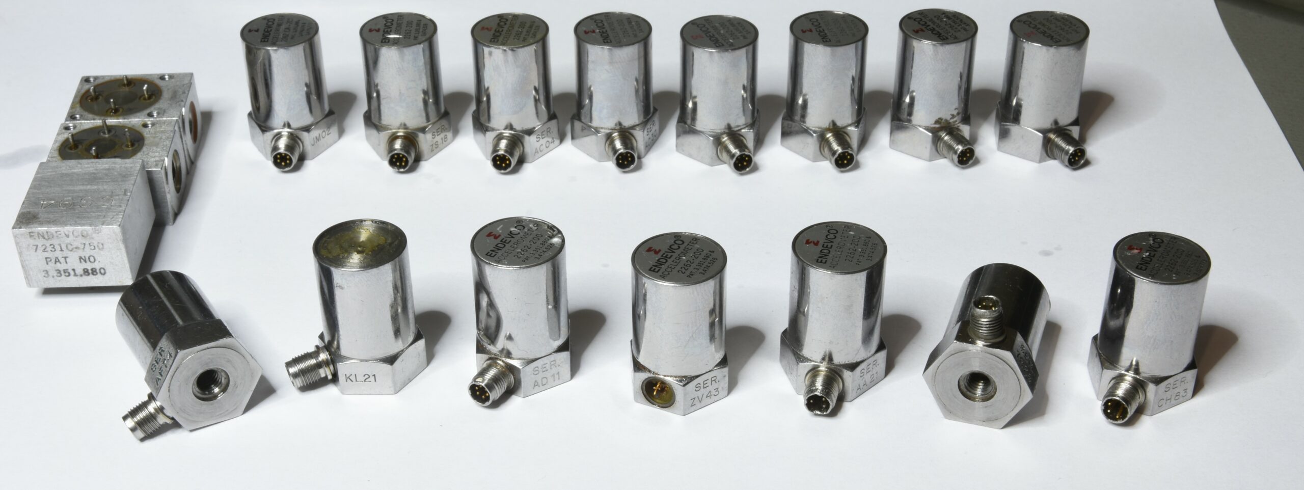
Just recently I’ve acquired a huge batch of piezoelectric accelerometers in an unknown condition which need to be tested for functionality. The goal of this project is to develop a small prototype calibration device in order to be able to calibrate piezoelectric accelerometers by comparison method.
Piezoelectric Accelerometers
Working Principle
Piezoelectric (PE) accelerometers are basically “acceleration-to-charge” transducers. They rely on the piezoelectric effect which – in simple words – converts mechanical energy into electrical energy. A piezoelectric transducer consists of a piezoelectric material (e. g. quartz, lithium niobate) and a small seismic mass.

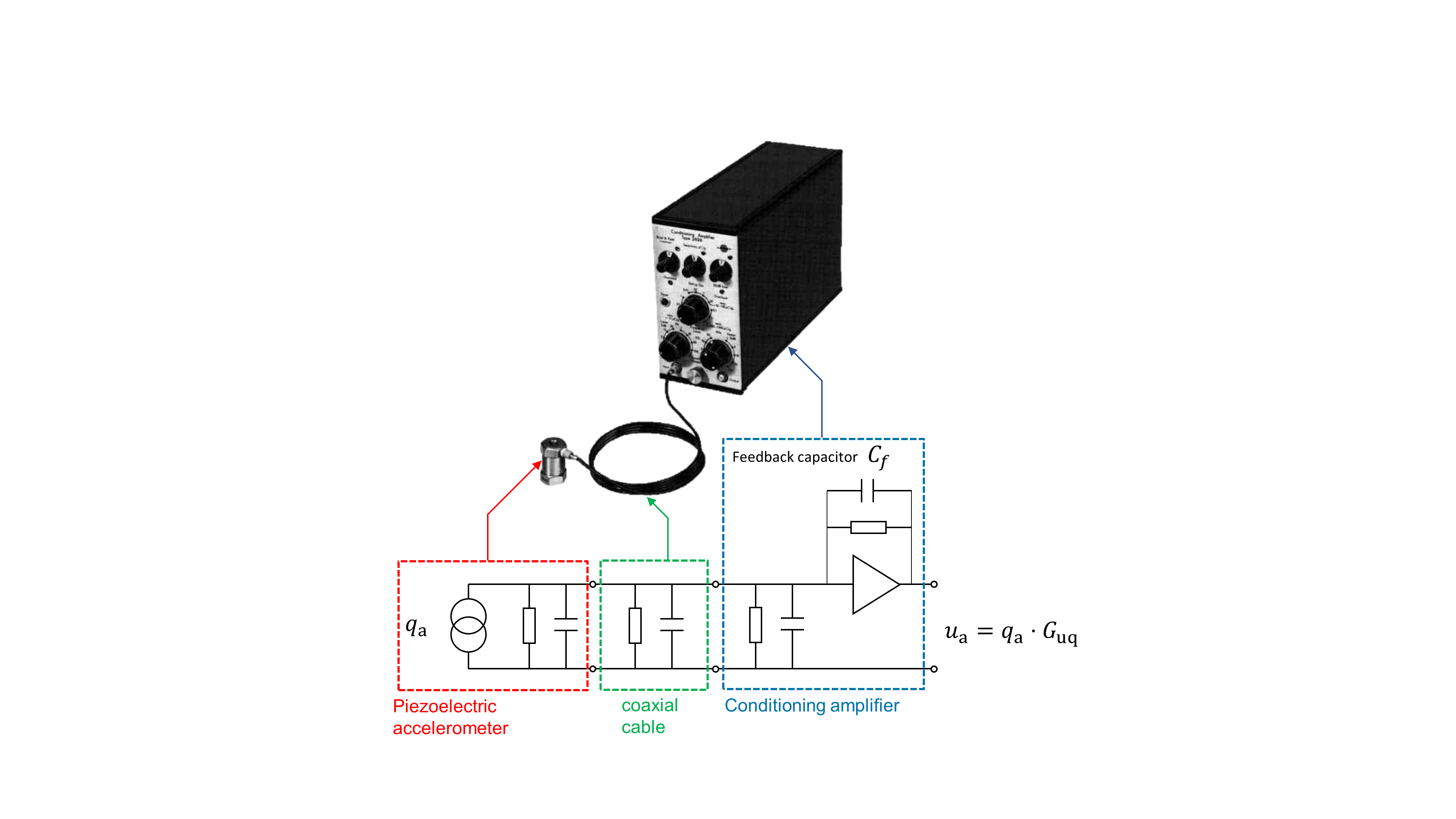
As soon as dynamic forces act on the spring-mass-system along the acceleration-sensitive axis, mechanical stress is introduced on the piezoelectric material which is mounted inside of the accelerometer housing (see Figure 2). The resulting deformation of the PE material causes a polarization which in return generates a change in surface charge density. The change in surface charge density is directly proportional to the mechanical stresses (e. g. force or pressure) and therefore proportional to the acting force or acceleration (if you remember the Newton’s 2nd law \( F = ma \longrightarrow a = F/m \)). The resulting change in surface charge density can be detected, amplified and converted into a measurable voltage with a proper signal conditioner or so-called “charge amplifier”. For simplicity’s sake I’ll refer to “charges generated by the accelerometer” instead of “polarization and change in surface charge density of the PE material”.
Harmonic Oscillator
From a mechanics point of view, the basic construction of a PE accelerometer can be approximated as a spring-mass-system with a low dampening as shown in Figure 3.

The harmonic oscillator is a very basic physical model of a spring-mass-dampener system. The huge advantage of this model is its simplicity: the harmonic oscillator equations contain the Newton’s laws of motion (\(F = ma\)) and Hooke’s law (\(F = kx\)) which can be solved analytically using so-called differential equations. While I’m skipping the mathematics part here and just want to mention that in reality things are more complex, some of the results of the differential equation for a driven harmonic oscillator are shown in Figure 3. Applying oscillations on a spring-mass-dampener system leads to the curves (Bode plots) showed in Figure 3. One of critical parameters of a harmonic oscillator is the natural frequency \(\omega_\mathrm{n}\). It’s a particular frequency where the spring-mass-system is oscillated (or “shaken”) in resonance, e. g. the mechanical system responses with very large displacement amplitudes while being excited by very small amplitudes. Resonance phenomena can be experienced in everyday situations like music instruments, swinging bridges, vibrations in cars driving at certain speeds, tuning forks etc.
For example, sinusoidal excitations of an accelerometer at its resonance frequency can lead to damage or change of its specified properties, e. g. sensitivity. A high resonance frequency is achieved by using stiff material (spring constant \(k\) should be high) and small seismic mass. In case of an accelerometer, the resonance frequency should be as high as possible, usually in the order of 30…50 kHz for high-frequency or shock measurements. Brüel & Kjaer suggests in [1] that the typical useable frequency range of an accelerometer is specified to approx 30% of the natural frequency.
The equation \( \omega_\mathrm{n} = \sqrt{k/m} \) for the undamped natural frequency suggests that using no seismic mass would lead theoretically to an infinite natural frequency! In reality, we need a small seismic mass – it has to be just big enough so it can compress or tension our spring (which is basically the PE material) through its inertia. We need to create mechanical stresses on the PE material in order to generate our precious charges. Basically a larger seismic mass leads to a larger signal output which is exploited in the low-frequency range (\(f \ll 10 ~ \mathrm{Hz}\)) and in seismometers.
Measuring Accelerations with a PE Accelerometer
The amounts of charge generated by an PE accelerometer are very minuscule. In order to get a measureable amount of charge, the PE elements are stacked in parallel as seen in Fig. 1. We’re talking about tens to hundreds of femto-Coulombs (fC) per m/s² of acceleration up to few pico-Coulombs (or pC) per m/s². Typical values are in the order of few pC where \(1~\mathrm{pC} = 10^{-12}~\mathrm{A} \cdot \mathrm{s}\). Just imagine charging a small capacitor with a capacitance of C = 100 pF and a voltage of U = 0.1 V and you will get according to the capacitor equation \(Q = C \cdot U\) a value of \(Q = 10~\mathrm{pC}\). High-intensity accelerations in the order of 1 … 100 km/s² – which are found in crash or shock testing – may generate few nano-Coulombs of charge. Measuring such minuscule quantities requires a somewhat specialized test equipment: ultra low noise coaxial cables with limited length and a signal conditioner for impedance matching, signal amplification and filtering.
Calibration of a Piezoelectric Accelerometer
As soon as one buys (very expensive) acceleration measurement equipment, the new instruments will be factory calibrated and the manufacturer will provide calibration certificates to the customer. A calibration certificate contains important information how to establish the relationship between the input quantity (acceleration) and the output quantity (charge or voltage). This information is usually called sensitivity of an accelerometer. The sensitivity of an accelerometer is determined during a process called calibration. According to JCGM:200 (2012), the International Vocabulary in Metrology (VIM), a calibration is
[…] operation that, under specified conditions, in a first step, establishes a relation between the quantity values with measurement uncertainties provided by measurement standards and corresponding indications with associated measurement uncertainties and, in a second step, uses this information to establish a relation for obtaining a measurement result from an indication.
In other words: a calibration is a comparison between input and output quantities of any kind. The input quantity is provided by a well-known standard, the output quantity is provided by a device under test (DUT). In case of an PE accelerometer, the input quantity is an acceleration, the output quantity is charge (or voltage if using a conditioning amplifier).
Unfortunately – when buying surplus stuff – there is always a risk of getting either a defective or incomplete unit. The provided calibration certificates may be either wrong or got lost. Some PE accelerometers are well over 50 years old and may have drifted over time. For my purposes, I’ll have to skip the “measurement uncertainties” part for now because I want to test the accelerometers for their qualitative condition and functionality. I’ll return to the metrology part in a future project.
Description of the Calibration
The calibration process is shown in a block diagram (Figure 5). In order to generate an acceleration \(a(t)\), we need to set our Accelerometer Standard (REF) and the Device Under Test (DUT) in an oscillating motion. This is usually done with an electrodynamic exciter – a technical term for “shaker” or “loudspeaker”. The working principle of an electrodynamic exciter is identical to the principle of the well-known loudspeaker. We’re generating a low distortion sinusoidal signal with a function generator which is fed into a power amplifier. The amplified signal drives the coil of the moving part inside of the exciter which in return creates the oscillating motion. Amplitude and frequency of acceleration are set by the function generator, which are typically in the range from 10 Hz to 10 kHz and 1 m/s² to 200 m/s². The frequency and amplitude ranges depend strongly on the construction of the electrodynamic shaker and the total weight of the DUT and REF accelerometers.

The shown equation might look scary and complicated but it’s pretty straightforward: we’re measuring the output voltages of both measuring chains and multiplying their ratio with the charge sensitivity of our reference accelerometer (\(S_\mathrm{qa,REF}\)). Afterwards we’re multiplying the resulting expression with the ratio of transfer functions of our charge amplifiers (\(G_\mathrm{uq}\)), which have to be determined by a different type of calibration. For the sake of completeness, I would like to mention that the sensitivities and transfer functions in general are complex values (e. g. \( \underline{S}_\mathrm{qa} = |S_\mathrm{qa}| \cdot \exp{(\mathrm{j}\omega t + \varphi_\mathrm{qa}}) \)) and we’re dealing with the magnitude \( |S_\mathrm{qa}| \) of the complex transfer function. I’ll try to cover this in a future blog post.
Experimental Setup
Since we need to perform the measurements over a wide set of frequencies, it is highly recommended to automate the task as much as possible. The instrument control, data acquisition and data analysis can be done with a PC. I’m using Python 3.9 with pyvisa, pandas and numpy on a Windows 10 machine. My accelerometer reference standard is a Kistler 8076K piezoelectric back-to-back type accelerometer. For the purpose of this experiment, I’ve tested two different PE accelerometers: Brüel & Kjaer 4371 and Endevco 2276, which are so-called “single-ended” accelerometers. Single-ended type accelerometers can be mounted on the top of a back-to-back type accelerometer and therefore calibrated by comparison method. The vibrations are generated by a Brüel & Kjaer 4809 electrodynamic exciter which is connected to a Brüel & Kjaer Type 2706 Power Amplifier and an Agilent 33250A frequency generator. I’ve used two charge amplifiers for the accelerometers, basically Brüel & Kjaer Types 2650 (REF) and 2635 (DUT). They were connected to HP 34401A digital multimeters. AC voltage measurements were performed in “ACV mode” which outputs the root mean square (RMS) voltage of the respective measurement chain signal output. An oscilloscope can be used to monitor the output waveforms in order to detect unwanted noise and distortions. This is a small downside of RMS measurements: the DC offsets and noise fully contribute to the measurement result.

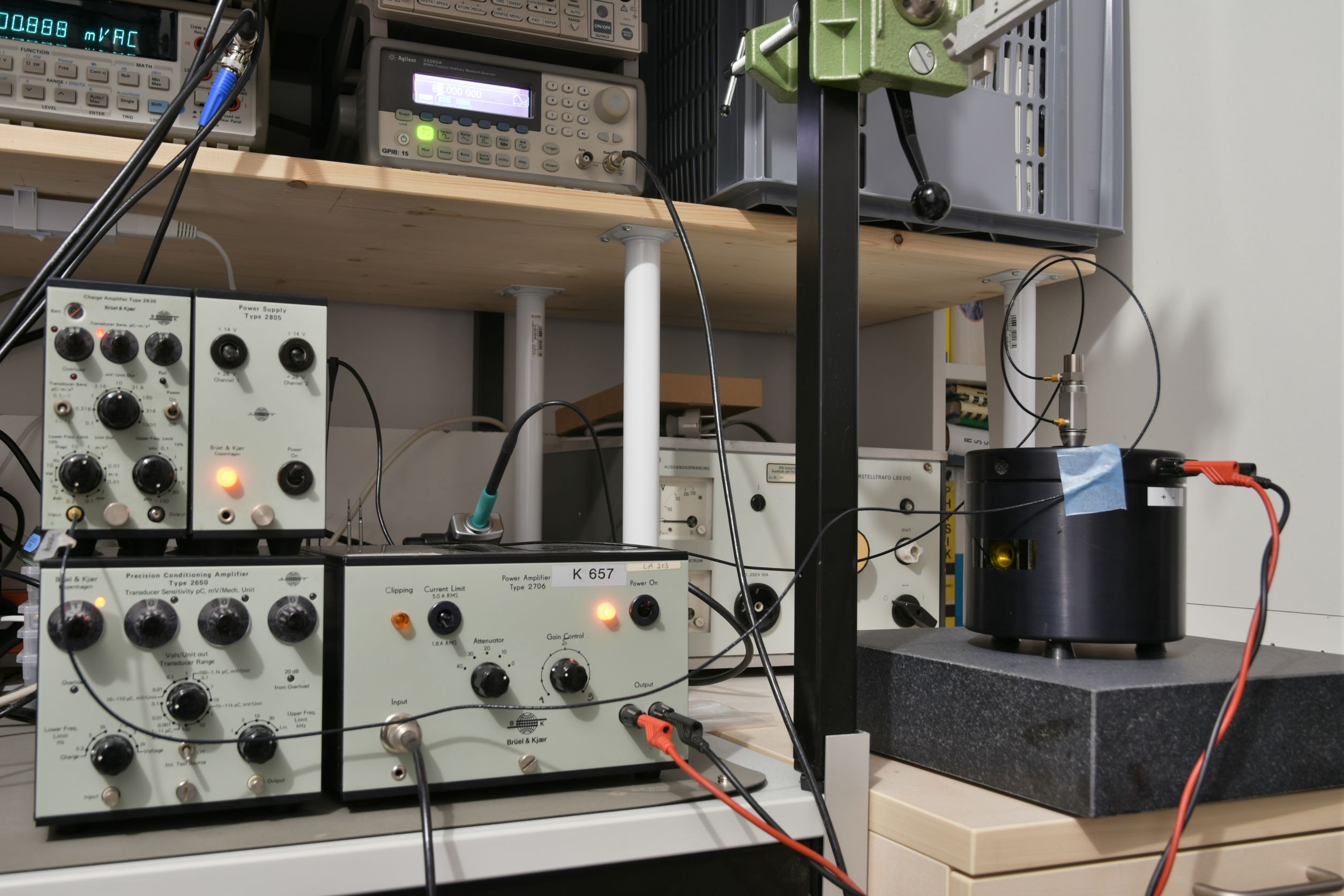


Setting up the devices wasn’t very difficult. The electrodynamic exciter needs a stable and massive base along with an adequate vibration isolation. If the vibration isolation is neglected, the vibrations are coupled into the desk and into the building. Using hard foam between the desk and granite block proved being very inexpensive and efficient. The support for low noise cables are also improvised. The cable mounting is a major source of experimental errors. Due to the triboelectric effect, a bending or vibrating coaxial cable also generates charges which are superimposing the measured accelerometer signal. In short words: the reference accelerometer is measuring a slightly higher acceleration than expected. Therefore the sensitivity drops due to \( S = q/a\). This can be seen in the measurement results at frequencies below 25 Hz. At higher frequencies (e. g. > 25 Hz) the displacement amplitude of the vibration becomes very small and the triboelectric effect becomes negligible. I’ve used a torque wrench with 2.0 Nm and the contact surfaces were slightly lubricated in order to prevent deviations at higher frequencies (>5 kHz).
Measurement Results

The calibration result can be seen on the left hand side in Figure 6. The top curve represents the charge sensitivity of the DUT plotted vs. excitation frequency. There are some deviations in the frequency response which are really annoying but I’m really satisfied with the overall result. Calculations of the relative deviation of the charge sensitivity at a reference frequency of 160 Hz can be compared with the data provided by the manufacturer. A 5% deviation at 6 kHz is in a good agreement with the specifications! My measurements show even higher deviations at frequencies f > 6 kHz so there must be some kind of systematic error which has to be investigated. Nevertheless, the measurement is automated and it takes approx. 5 minutes for a “sweep” of 31 discrete frequencies in the range from 10 Hz to 10 kHz. I’ve used standardized frequencies which are known as Third Octave Series according to ISO 266. The bottom graph shows the acceleration amplitude over the frequency range. I’m ramping up slowly in order to minimize distortions. A limit of 20 m/s² is set for noise reasons in my apartment – the generated sine tones can be very annoying and I don’t want to wear ear protection all the time.
Summary and Conclusion


This project clearly is a success! It took much time and effort in order to get the experiments straight and to automate the measurements. I was able to perform a calibration of a piezoelectric accelerometer with decent quality equipment. The results are “not bad” although I see much room for future improvements. I’ll have to improve the measuring chains and eliminate noise sources. I’d like to improve the Python code and generate a Graphical User Interface (GUI) for calibration purposes. Playing with a HP 3562A Dynamic Signal Analyzer was also very fun! I was able to dump the FFT measurement data (Thanks to Delrin for his Python hint!) via GPIB and didn’t rely on photographs of the display. A little downside of this instrument is its loudness and electricity consumption in the order of 400 W. I’ll certainly use the signal snalyzer during the winter months in order to heat my apartment 😉 I’m literally scratching on the surface in the fields of vibration measurements and the future will bring more interesting projects. The ultimate goal is to build a laser interferometer as an acceleration reference standard and to estimate the uncertainties of the built calibration devices.
References
[1] Serridge and Licht, Piezoelectric Accelerometer and Vibration Preamplifier Handbook, Brüel & Kjaer Naerum, Denmark, 1987
[2] Methods for the calibration of vibration and shock transducers – Part 21: Vibration calibration by comparison to a reference transducer, ISO 16063-21:2003
[3] Richtlinie DKD-R 3-1, Blatt 3 Kalibrierung von Beschleunigungsmessgeräten nach dem Vergleichsverfahren – Sinus- und Multisinus-Anregung, Ausgabe 05/2020, Revision 0, Physikalisch-Technische Bundesanstalt, Braunschweig und Berlin. DOI: 10.7795/550.20200527
Calibration of a Piezoelectric Accelerometer by Comparison to a Reference Transducer Read More »