I spent the past weekend primarily with chores. I ordered some nice ESD-protected boxes in order to store all of my sensitive components which are mostly used for my electronics and optics projects. The cleaning of my apartment was a full success and I’m happy with the results.
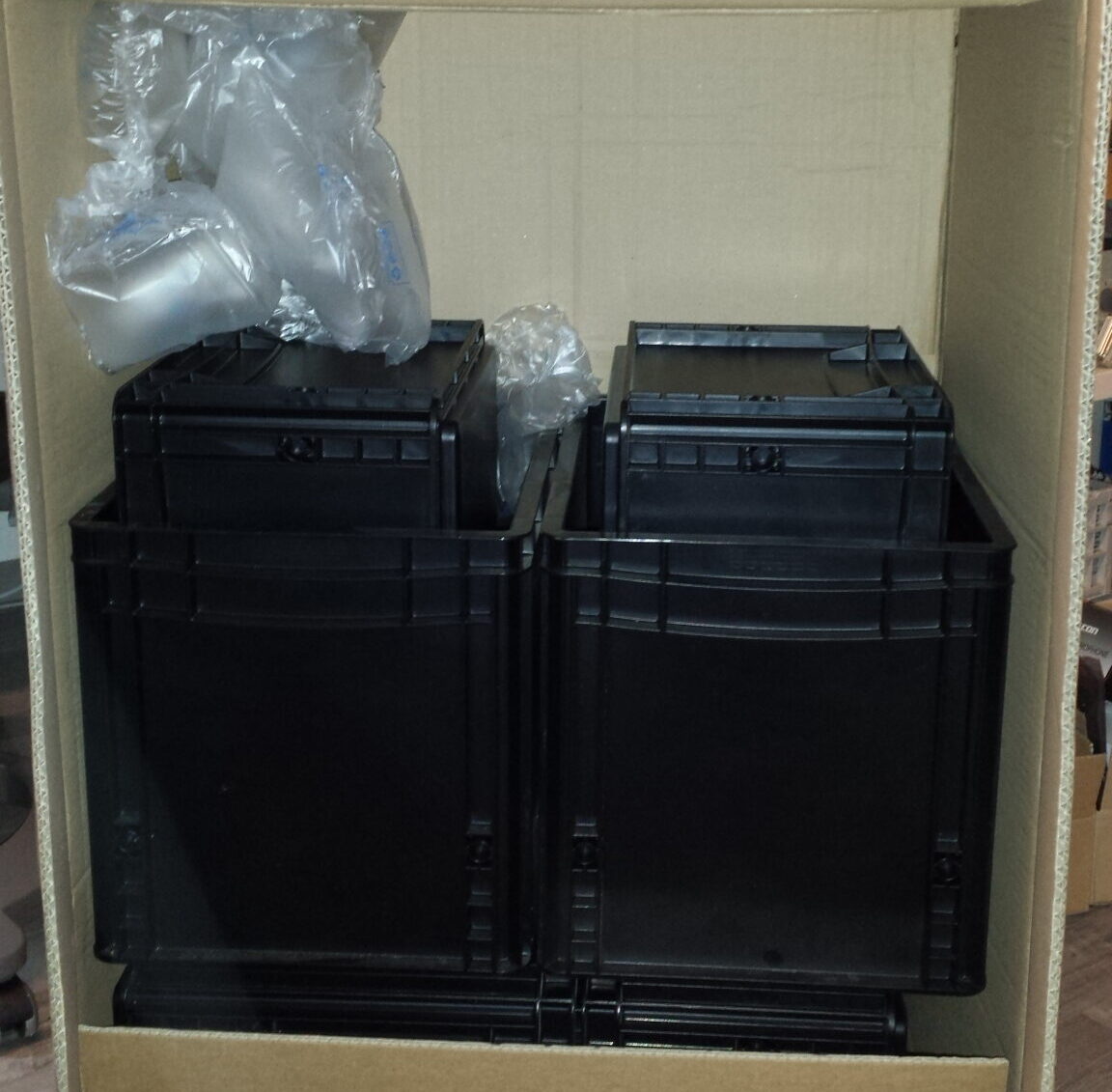
My newly ordered ESD boxes. Size: 40 cm x 30 cm x 22/30 cm.
I also spent some time upgrading my old PC for a future project. Approx. 12 years ago, I bought a second hand PC from a German reseller called ITSCO for about 450 EUR. It’s a workstation PC, type Dell Precision T5400 (2x Intel Xeon E5440 2.83 GHz, 4096 MB RAM (DDR2 667 ECC Fully Buffered, PC2 5300F), DVD-RW+ and whatnot). It was my daily workhorse until 2021. Using a PC for 11 years is quite impressive if compared to older generation PCs from the mid-1990’s until ~2006. Those old PCs were prone to obsolescence because of Moore’s Law.
Over the years, I experienced only few minor problems with the Dell workstation: I’ve lost few RAM modules (error correction code memory, ECC) due to thermal issues. The RAM modules got pretty hot (70 °C – 80 °C) during operation. If one does not take care of dust and proper ventilation during hot summers, those electronic parts will inevitably fail. Luckily, the ECC DDR-SDRAM prices for those kind of PCs fell significantly over the past years so I was able to restock my RAM module supply with many replacement modules for a minor investment of ~20ish EUR.
Unfortunately, the user experience declined over time. Upgrading to Windows 10 and Google Chrome as a web browser in 2019 was a pain in the ass. Those applications are very power-hungry, especially when it comes to RAM. An average PC with 4-8 GB RAM – while being very decent in the years ~2010…2015 – is totally crippled by modern day software. Booting a PC and loading a web browser already consumes 4-6 GB or RAM! So I moved on and acquired another workstation (hp Z440) as an intermediate solution because of the ongoing global shortage of electronic components.
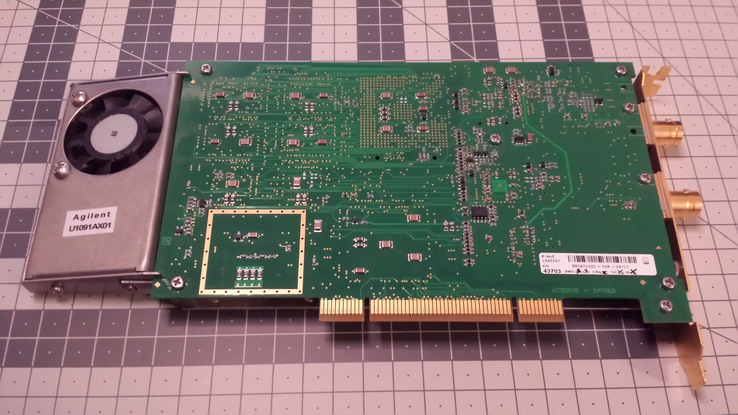
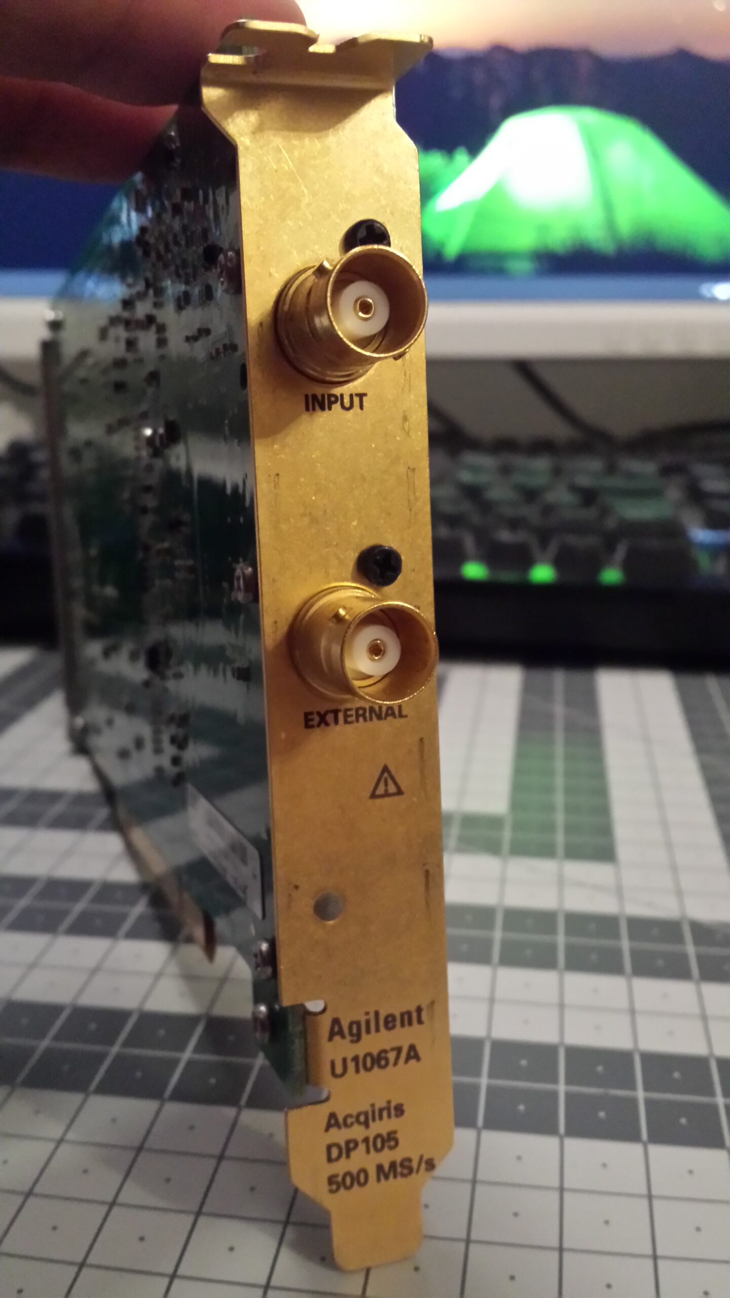
Nevertheless, my Dell workstation is still of great value! Due to its age, the motherboards from the 2006-2009 era were produced with PCI and PCI Express (x16). Modern day PCs and motherboards are produced with PCI Express slots exclusively although there are PCIe-to-PCI bridge solutions out there. While PCI slots are becoming more and more obsolete, there is still valuable hardware out there which is based on this kind of technology: PCI-based oscilloscopes. I bought over the past years such PCI oscilloscope cards which in return can be used as high-speed digitizers. A digitizer is a piece of test equipment which converts analogue signals (e. g. voltages) into digital ones. The digitized values are called samples. Digitized signals have one huge advantage: since the samples are basically just numbers, they can be treated numerically for further calculations! A digitized and recorded signal can be further processed, e. g.: arithmetic, regression analysis, spectrum analysis (FFT), waveform arithmetic and analysis, plotting, digital filtering, etc.. This will be very interesting for a super secret future project 😉
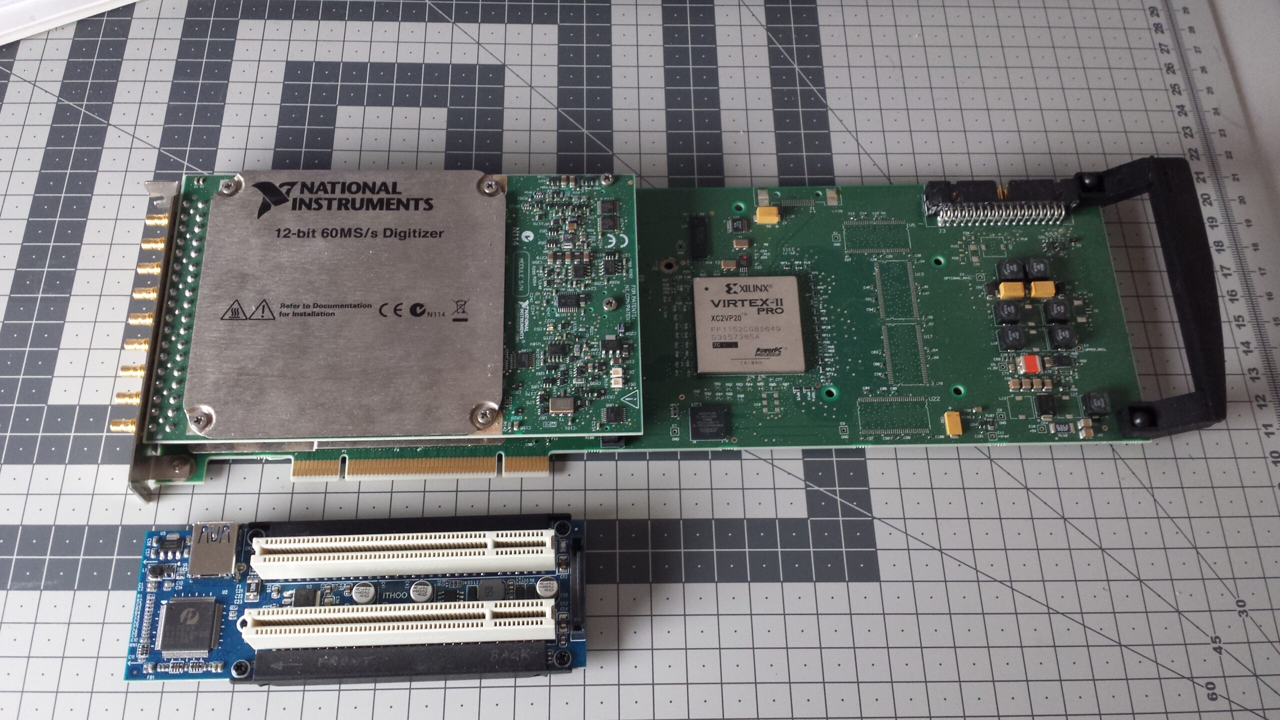
NI PCI-5105 digitizer card along with a two-slot unbranded PCIe/PCI bridge.
1 MHz Square wave signal captioned with Agilent/Acqiris oscilloscope software.
So in order to install two of those oscilloscope cards, I had to rearrange few cards. My old “gaming graphics card” (AMD Radeon 7700XT Series) had to be replaced by a smaller graphics card (Nvidia Quadro FX 580). The graphics card needed to be smaller in size because of the limited space inside of the PC housing and PCI/PCIe slot arrangement. After installing the oscilloscope cards, it is very necessary to leave space between card in order to prevent thermal failures by heat buildup. The oscilloscope cards may heat up in the order of 60 °C during operation and maybe up to 65 °C during data acquisition. If one does not take care of this issue, the cards may overheat and fail over time. I also cleaned the PC with air duster and a vacuum cleaner in order to clear the slots from dust.
Dell Precision T5400. A little bit dusty but after 12+ years still in a good shape!
Card arrangement inside of a Dell Precision T5400. The graphics card (that thingy with a black fan) had to be replaced.
National Instruments PCI-5105 8 Channel, 12-bit, 60 MS/s oscilloscope card.
Card arrangement after replacing the AMD Radeon two-slot graphics card with a Nvidia Quadro FX 580. Now both oscilloscope cards fit with proper clearances.
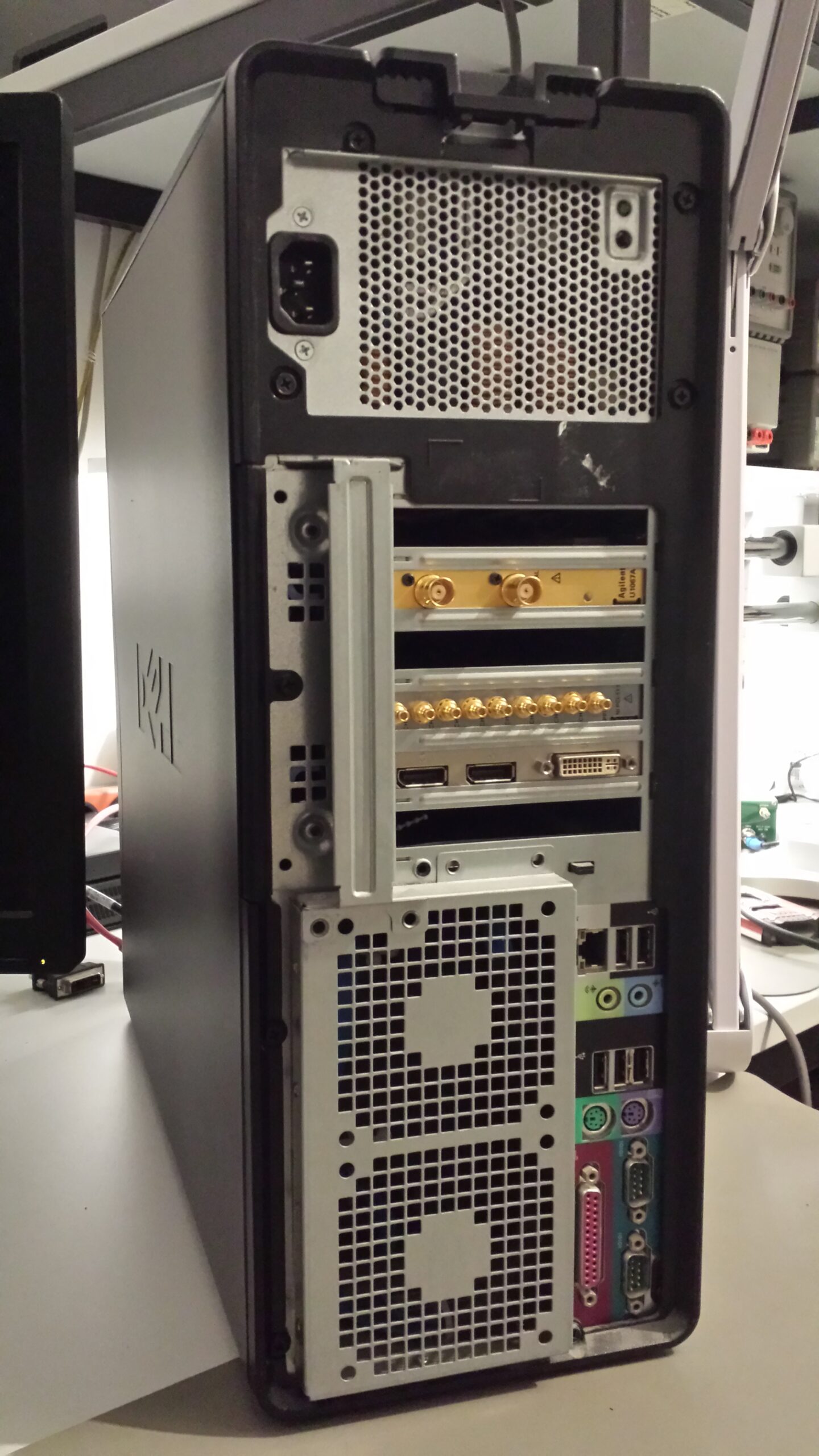
Rear side of the Dell Precision T5400 showing the oscilloscope cards.
Another “ancient” PC (HP xw4600) with PCIe and PCI slots. This will be useful for another set of PCI Data Acquisition cards.
I hope this workstation will last few more years. I have already found an external PCI solution. A friend of mine ordered an unbranded adapter from China (based on an IC type P17C9X) for a very low price of ~25 EUR. It’s a PCIe-to-PCI bridge which serializes the PCI signals and transmits them via a USB-like cable to a PC. Since the whole thing is standardized, no further Windows/Linux drivers are needed. This concept proved to work with few tested PCI cards (e. g. NI PCI-GPIB) where the power consumption is fairly low. However, the PCI oscilloscope cards need certain amounts of power (~25 W) during operation and therefore an external power supply is necessary. If the PCIe/PCI-bridge does not provide the amount of power needed, the PC will freeze and one will have to reboot the system in order to recover. This can be solved by attaching a Molex to SATA power connector from the power supply to the PCIe/PCI-bridge. The “Chinese “module does not work with full-length PCI cards as seen in the pictures. I’ll try to desolder the SATA connector and arrange it differently in order to avoid the collision.
This test setup consisted of two PCI cards and a PCIe/PCI bridge. The cards were recognized properly by a Windows 7 PC and worked without issues.
Another quick arrangement of the PCI cards.
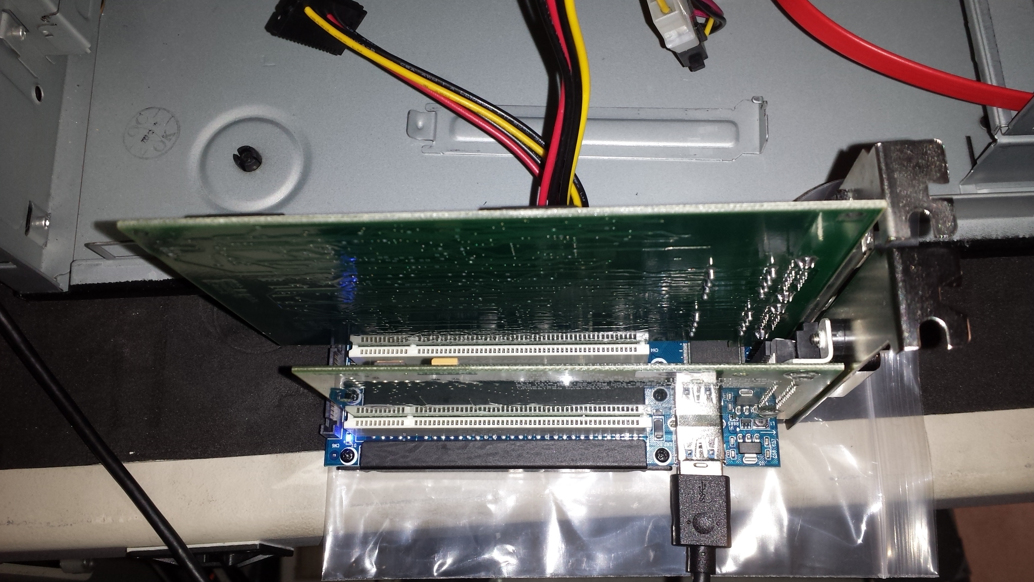
Photograph from the top (PCI cards on a PCIe/PCI-bridge).
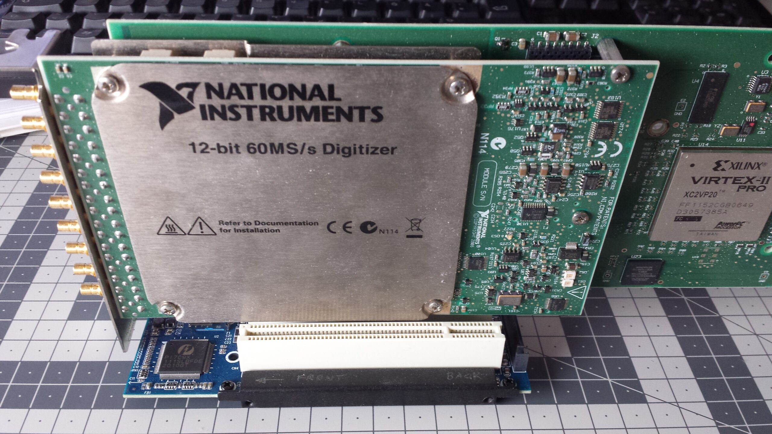
The NI PCI-5105 full-size card can be installed this way. But as soon as the PC does access the card, too much power is drawn. The power demanded can not be provided by the bridge alone. This leads to a PC freeze.
PCIe/PCI bridge with Molex-to-SATA adapters.
The full-length NI PCI-5105 does not fit properly. An additional power cord is needed to satisfy the power consumption, otherwise the PC won’t work properly.
While browsing the Internet, I stumbled here and there upon a nice little gadget for ham radio amateurs called NanoVNA. This is a compact Vector Network Analyzer (VNA) — a piece of test equipment which allows to measure radio frequency (RF) properties of a Device Under Test (DUT) such as Magnitude and Phase. This is very useful in order to characterize RF components such as antennas, filters, cables or amplifiers – the usual ham radio stuff. Few weeks ago I ordered a NanoVNA in order to perform simple tests on my RF equipment. This article will be about a quick set up of NanoVNA and doing some simple measurements.
Prices for “Maker/hobbyist level” VNAs vary from 50ish EUR to ~550 EUR (DG8SAQ VNWA V3) depending on model and additional accessories. More sophisticated vintage test equipment (HP/Agilent, Rohde&Schwarz) may be found on eBay in the range from 1k+ EUR to ~3.5k EUR. Brand new entry level VNAs start at ~2k EUR without upper price limit, depending on its measurement capabilities. As soon as you buy a VNA you will also need accessories such as torque wrench, lots of adapters (Type N to SMA to BNC and vice versa) and calibration standards (short/open/load/through, SOLT) in order to perform correct measurements. Professional calibration standards (e. g. metrology grade SOLT) are extremely expensive (~3…10k USD) and unaffordable for the low budget hobbyist – so yeah…
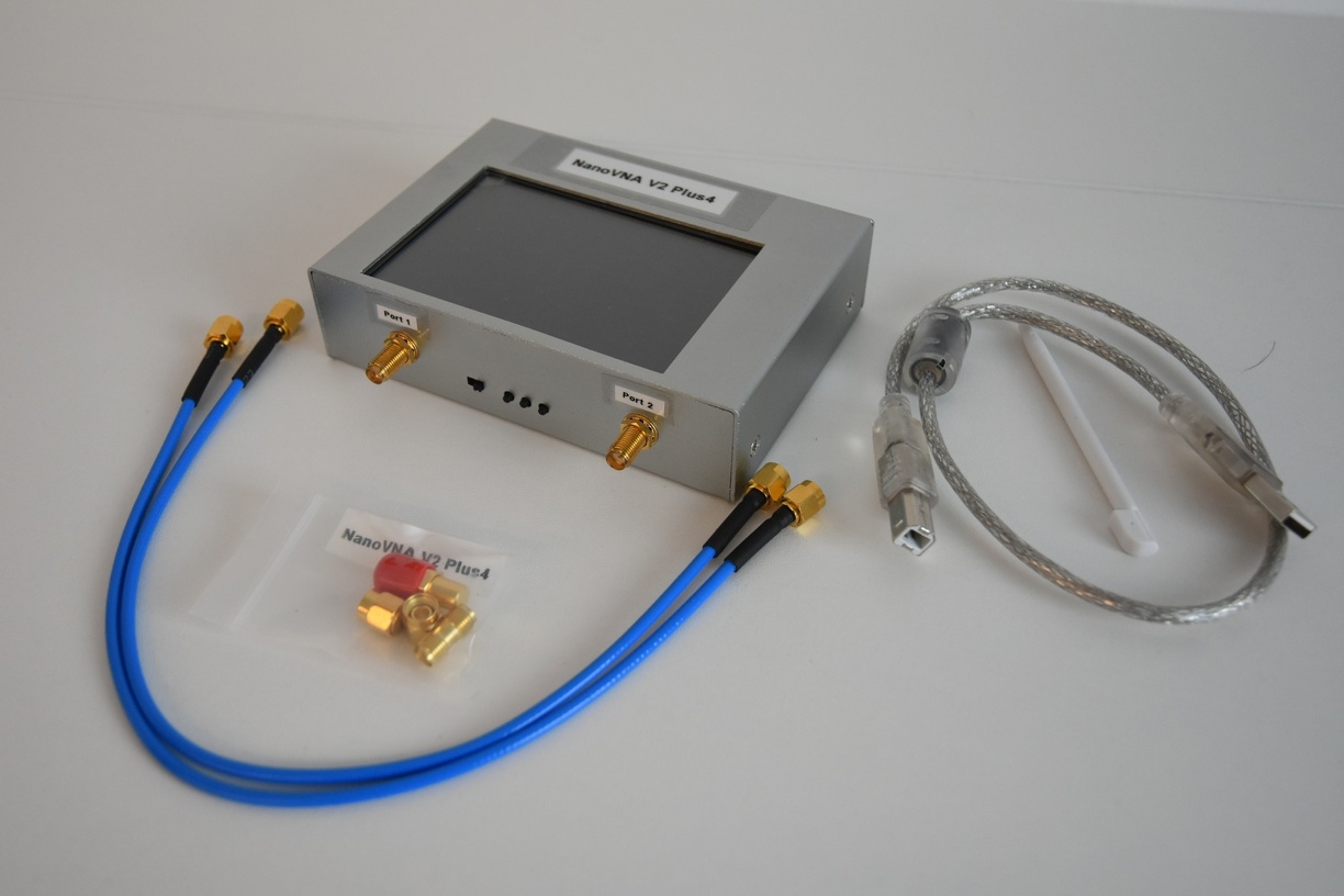
I didn’t want to spend 500+ EUR for a piece of test equipment which may result in even greater financial commitment. Based on the positive reviews and my requirements (easy to use, convincing measurements), I bought the NanoVNA V2 Plus4. It’s a compact 2-port VNA with integrated 4″ touch screen display, the specifications are listed here. The total price was ~215 EUR for NanoVNA + shipment + customs. The delivery from China to Germany took approx. 3 weeks from November till December 2021 (standard shipment, no express parcel).
The accessories are shown in the picture above: NanoVNA V2 Plus4 enclosed in a metal housing, two SMA cables, SOLT calibration set, USB cable and a small stylus for the 4″ touch screen. A 4/3 A type 18650 rechargeable Li-Ion battery was not provided due to transport restrictions of hazardous materials (exploding Li-Ion batteries on aircrafts…). The rechargeable battery had to be bought separately (+13 EUR). I’ve added few pictures of my NanoVNA V2 Plus4 here.
The usage of the VNA is pretty much straight-forward: turn it on, set sweep parameters, perform SOLT calibration and test your DUT. The basic measurement results provided by a VNA are Magnitude and Phase over the set frequency range. Those measurements are used to calculate very useful quantities such as VSWR (voltage standing wave ratio), ESR (equivalent series resistance), LCR (inductance, capacitance, resistance) and plotting a Smith chart. The result can be seen directly on the 4″ display and read by different cursors. This is a perfect tool to do quick performance or sanity checks on RF components.
As soon as one wants to do systematic measurements on different components, it becomes a little bit inconvenient to photograph the Smith chart due to glare, mirror reflections and possible motion blur while taking photographs. However, it is possible to control the NanoVNA via USB and read out the measurements to the PC. The readouts can be stored and processed via standard software such as MS Excel, LibreOffice Calc, Python/matplotlib, MATLAB, GNU Octave and others. This is where the fun begins.
NanoVNA readout via USB
An user from the EEVBlog (joeqsmith) tested early versions of NanoVNA and was quite unhappy with the provided tools at the time. He developed a very useful software front end for the NanoVNA which is based on LabVIEW 2011. In his software, commands are sent via USB protocol to the NanoVNA in order to set measurement parameters and to perform SOLT-calibrations. After triggering the measurement, the data is transferred to to PC and displayed graphically and processed through math equations. He put a lot of effort in the development and the results are astonishing. His software is capable of controlling NanoVNA via comprehensible user interface, taking measurements, performing calibrations, calculating almost all imaginable RF quantities in time and frequency domain. This is very helpful for newbies like me who have never worked with a VNA before. His software can be found on GitHub, downloaded and used freely with no limitations or charge. Props to joeqsmith — he maintains an active and educational YouTube channel so check it out if you’re interested in RF or handheld Digital Multimeter testing methods.
First steps
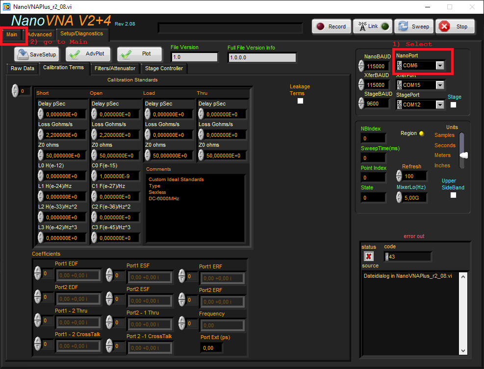
Buy NanoVNA, plug in the USB cable and turn it on. If you’re using Windows 10, the device should be recognized as USB CDC (Communications Device Class) on a virtual serial port (e. g. COM6). Next steps will be a little bit annoying: create an account on the National Instruments (NI) homepage, download and install the NI LabVIEW Runtime Engine (Version 2011 SP1 32-bit, size ca. 215 MB) and NI VISA. I have installed VISA v17.0 which is a 750 MB chonker. It contains drivers for USB/Serial communications any many others (also some important drivers for my obsolete GPIB test equipment which aren’t supported in the newer versions anymore). Install VISA and the Runtime Engine and spend your precious life with many reboots. I highly recommend to read Joe Smith’s User Manual, otherwise you may run into problems. Unfortunately, NI software is closed source/BLOB but everybody is encouraged to develop his own free and open source software for NanoVNA.
After the Installation is complete, download, extract and run the Runtime Version Executable (NanoVNA_V2Plus.exe) from Joe’s GitHub. Execute the File (abort the file dialogue if you don’t have any stored calibration files) and you should see something similar to the screenshots below. Setup the connection parameters (COM-port) and establish a link to your NanoVNA.
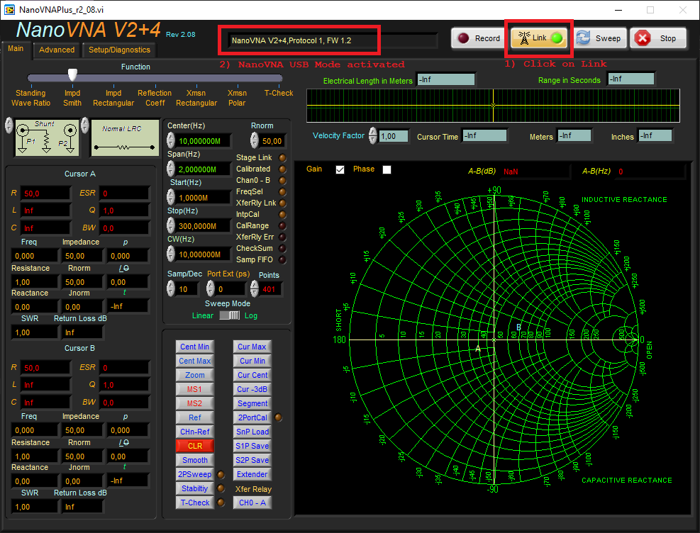
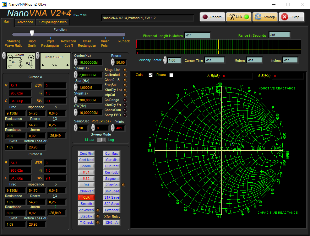
After starting NanoVNA V2+4, one needs to select the proper COM Port. Switch to “Main” tab afterwards.Click on the “Link” button and your NanoVNA should display “USB Mode”. The NanoVNA identifier message should appear.Photograph of the NanoVNA V2 Plus4 in the USB Mode.Start the sweep by clicking on the “Sweep” button. One should see some activity during the sweeps. I’ve connected a 50 Ohm load on Port 1 as seen in the Smith chart.
Alright, now we’re ready to go. Next step: SOL(T) calibration, taking measurements and data analysis. The usage of this software is described in Joe Smith’s User Manual or on his YouTube channel. He has a plenty of demonstration videos how to make proper measurements with NanoVNA V2 Plus4. This is easily done by clicking on the “2PortCal” button followed by some dialogues. After the SOLT calibration is performed, it can be saved and reused. A calibration is necessary as soon as the frequency span changes.
Sanity Tests
It’s a good practice to somehow validate your measurements. This requires some additional gadgets like filters or self-made circuits. I’ll gather some over time. I’m currently checking if the attached SOL standards are displayed correctly.
Testing a coaxial cable
50 Ohm coaxial cables such as RG58 or RG174 are widely used as transmission lines for radio frequency signals. Some important electrical properties of this cable type are: characteristic impedance (typical 50 ± 2 Ohm), capacitance per unit of length (96 pF/m), attenuation per unit of length (0.67 dB/m) and its operating frequency range (DC – 1 GHz). Data taken from Radiall’s RF and Microwave assemblies. For amateur radio operators, the SWR (standing wave ratio) is another important quantity which determines the match between impedances of the source (e. g. transmitter) and the load (e. g. an antenna). In case of an impedance match Z = Z_0, we obtain a SWR close to 1:1. We can measure the impedance Z with a little help of a VNA over a wide frequency range.
NanoVNA measurement setup. DUT: Tektronix 012-0482-00 Precision Coaxial cable. Inside of the cable loop are my BNC “calibration standards”.
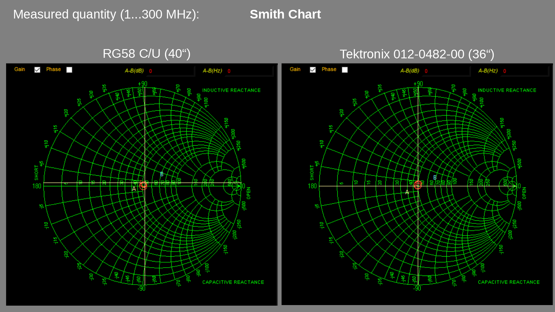
This is what the measurement setup looks like. I’ve connected the NanoVNA ports to two SMA cables (blue) in order to perform a SOLT calibration. My DUT will be a Tektronix 012-0482-00 Precision Coaxial Cable which has a length of 36″ and an impedance very close to 50 Ohm. I’ll set up the measurement for 1 MHz to 300 MHz and check the SWR, attenuation/losses and its impedance. The measurement results can be seen in the figures below.
Measurement result: Smith Chart. Comparison between two coaxial cables of slightly different lengths. Frequency range: 1 MHz to 300 MHz.Measurement result: Transmission Rectangular. Comparison between two coaxial cables of slightly different lengths. Frequency range: 1 MHz to 300 MHz.Measurement result: Standing Wave Ratio (SWR). Comparison between two coaxial cables of slightly different lengths. Frequency range: 1 MHz to 300 MHz.Measurement result: Reflection Coefficient. Comparison between two coaxial cables of slightly different lengths. Frequency range: 1 MHz to 300 MHz.Measurement result: Impedance Rectangular. Comparison between two coaxial cables of slightly different lengths. Frequency range: 1 MHz to 300 MHz.
Conclusions
There you have it! Both cables show a similar performance. Tektronix 012-0482-00 shows an impedance slightly closer to 50 Ohms and a slightly better transmission compared to a no-name brand RG58 C/U. Well, maybe the sharp drop of the reflection coefficient coincides with the fact, that this cable has to be used along with Tektronix SG 503 Levelled Sine Wave Generator in order to perform oscilloscope bandwidth checks. Tek SG503 covers the frequency band from 250 kHz up to 250 MHz. Very interesting! Maybe this information may be useful to other Tektronix users. I’ll try to characterize the Tektronix coaxial cable with a “slightly better equipment” later this year, just to validate the NanoVNA measurements. Please take the provided information “as is”. It might be wrong after all.
NanoVNA – would recommend
The NanoVNA is a very useful, nice and affordable addition to a hobbyist electronics lab. Using Joe Smith’s NanoVNA software works pretty well and offers a rich repertoire of calculations and graphical diagrams. I didn’t experience any kinds problems on my Windows 10 machine while using Joe’s software. The installation and setup was straightforward and I was able to obtain plausible measurements. Unfortunately I don’t have coaxial cables with matching lengths in order to make comparison measurements with my Tektronix 012-0482-00 but that’s the part where one starts going down the RF rabbit hole…
Few things to consider
Please be aware that the components used in combination with NanoVNA are very cheap. The quality is “OK” or let’s put it in another way: “good enough for the job”. The devil is in the details. In order to perform reliable and comparable measurements, one needs quality cables, good connectors, good adapters, better calibration standards and a torque wrench. If you’re possessing good RF gear, please be careful when interchanging the components. It’s very easy to damage quality gear with cheap rubbish. I’m trying to maintain two ecosystems: the cheap components will be used for non-critical projects and quick and dirty measurements. The quality equipment will be used for careful measurements and calibration.
Going down the RF rabbit hole?
What if one already possesses quality accessories — a question might arise why not spending money on a good vintage VNA anyway? Unfortunately I’m not an RF engineer and I don’t test or develop commercial RF circuits. RF is just a hobby and not my daily business. This kind of affordable tool lets you make a first step into the world of RF components and circuit testing. I don’t need to emphasize its usefulness for testing and debugging of RF circuits or performing sanity checks. I’ll keep looking for a vintage HP/R&S VNA because the answer to this question is always YES.
During the past year and a half, I’ve build my electronics lab. I’m able to measure many electrical quantities like voltage, current, resistance, capacitance, inductance, frequency, spectra and much more. I surely am suffering to the Gear Acquisition Syndrome and I’ve already posted some pictures inside of the TEA-thread (Test Equipment Anonymous) of the EEVBlog. I wasn’t kidding when I posted that I have sold my soul for Tektronix. I’d like to start restoring/repairing/calibrating/maintaining the older Test Equipment in order to do be able to do some exciting electronics projects in the years to come!
After half a decade of changing jobs, cities, apartments, relationships, … — I think it’s time to finally follow my passions and share them with like-minded people 🙂