Controlling Test Equipment via GPIB and Python
Introduction
Taking measurements with electronic equipment doesn’t require much skill and effort: turn the device on, set up the measurement parameters such as input channel/range/sensitivity, trigger the measurement and read the numbers on the screen (if there are any). The same procedure can be applied in everyday situations – whether you have to read the time from a clock or check the temperature in your fridge/oven.
But what if one does have to take thousands or even million of measurements every day? What happens if measurements have to be performed 24/7? There surely are applications where it is necessary to take measurements manually but putting a human behind a bench and performing boring and repetitive measurements during a 8-hour-workday is prone to exhaustion and errors. This is where automated test equipment (ATE) kicks in. It is possible to let a computer do the “boring stuff” while the human operator may spend his or her precious time on solving problems instead of doing repetitive work. I’ve successfully stolen borrowed and tested foreign Python code and want to demonstrate how to control a digital multimeter and a function generator via General-Purpose Interface Bus (GPIB) and Python’s pyvisa module.
GPIB
GPIB is a 8-bit parallel interface bus which has been invented in the late 1960’s by Hewlett-Packard (see Wikipedia article). Prior to its standardization in the late 1970’s as IEEE 488, it was known as HP-IB (Hewlett-Packard Interface Bus). It allows interconnection between instruments and controllers. It is system independent of device functions. This de facto standard has been around for a while and is well established in the Test & Measurement industry. Fast forward to the year 2022, GPIB is still present in test equipment although in recent two decades, communication with instruments have been enabled with modern-day interfaces such as USB or Ethernet. GPIB allows a very diverse topology – one can connect all instruments either in a Daisy Chain or parallel configuration or even in a combination of both of them. There are certain GPIB-specific limitations concerning cable lengths, maximum number of connected devices, data transfer speeds and others which have to be considered when automating test equipment.
Experimental Setup
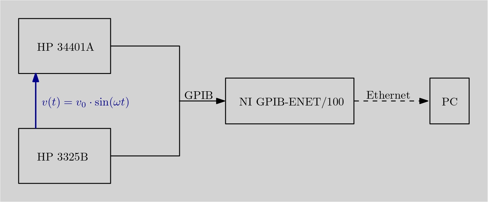
I’ve connected a HP 34401A digital multimeter to a HP 3325B function generator in order to generate a sinusoidal test signal, which can be represented by an equation \(v(t) = v_0 \cdot \sin (\omega t) \) with \(\omega = 2\pi f\). Both instruments are connected to a GPIB controller National Instruments GPIB-ENET/100. The GPIB-ENET controller acts as a bridge and allows communication to GPIB devices via ethernet, which is highly convenient in my lab. It allows me to control the instruments via LAN from any of my computers. This device requires drivers from National Instruments so I’ve chosen NI MAX v17.5 along with NI-488.2 driver in order to be able to use the legacy GIPB-ENET/100 controller. I’m using Windows 10 along with the WinPython distribution. WinPython comes along with Python 3.9.10 and hundreds of useful modules, such as numpy, pandas, matplotlib etc. (which are optional). The pyvisa module needs to be installed manually via pip, see PyVISA’s project website for further installation instructions.

Important notice for new users
Many of the GPIB-USB adapters sold on eBay are fakes or counterfeits. They are sold very cheap (different brands such as National Instruments, Agilent/Keysight, Keithley) in the price range of 100 EUR to 120 EUR per piece whereas the genuine GPIB-USB adapters often cost more than 400 EUR. Buying a new unit directly from the manufacturer will cost in the order of 900 -1200EUR which is kinda crazy! Nevertheless, some of the fake GPIB-USB adapters seem to work pretty well and are recognized by the official drivers. However, some EEVBlog users also report having problems with fake adapters… So it’s really a gamble.
I’ve bought a 2nd hand “fake” GBIB-USB-HS for cheap which didn’t work for the previous owner but works perfectly on my Windows 10 machine. I haven’t tested it with Raspberry PI yet which will be done in a future project. The GPIB-ENET/100 unit is a little bit pricy (~200ish EUR) but the most affordable interface cards are the PCI-GPIB types. I’ve seen genuine units being sold on eBay for 40-80 EUR. No need to spend hundreds of Euros for a GPIB interface. Microcontroller-based GPIB-USB projects also exist where one can assemble a GPIB-USB or GPIB-LAN controller for cheap (which may not work always but gets the job done). Proper GPIB-cables can be expensive, too, but I’ve seen them being sold for approx. 7 … 12 EUR per piece occasionally. Custom-made GPIB cables out of ribbon cable and Centronics/Amphenol connectors may also work and get the job done.

Example Code
First of all we’re gonna need to import some Python modules. pyvisa is mandatory, other modules will be useful.
# Import Python modules
import pyvisa
import numpy as np
import pandas as pd
import matplotlib.pyplot as plt
import datetime
import time
Next step: we need to open the pyvisa Resource Manager. We need to know the GPIB addresses of our instruments. For example, I’ve assigned GPIB address No. 4 to my digital multimeter dmm and the frequency generator fgen has the GPIB address No. 18. GPIB 22 is another digital multimeter which isn’t used in this example.
# Open pyvisa Resource Manager, print out a list with active devices
rm = pyvisa.ResourceManager()
print(rm.list_resources())
The print(rm.list_resources()) statement gives us the GPIB addresses of the connected devices, such as: ('ASRL3::INSTR', 'GPIB0::4::INSTR', 'GPIB0::18::INSTR', 'GPIB0::22::INSTR'). Now we can open a connection to the resources.
# Assign GPIB address 4 to dmm and open resource
dmm = rm.open_resource('GPIB0::4::INSTR')
dmm.read_termination = '\n'
dmm.write_termination = '\n'

# Assign GPIB address 18 to fgen and open resource
fgen = rm.open_resource('GPIB0::18::INSTR')
fgen.read_termination = '\n'
fgen.write_termination = '\n'
The dmm and fgen objects have been created. The statements dmm.read_termination = '\n' deal with line feed and carriage returns. The next step will set the DMM settings and call an identify string via a SCPI command *IDN?
# Set the DMM for measurements
print(dmm.query('*IDN?'))                      # Identify string
print(dmm.write('CONF:VOLT:DC 10,0.001'))      # Set DC voltage range and 4.5 digits of resolution
The same commands are applied to our frequency generator. The output of the DMM looks something like (name, model, firmware version):
HEWLETT-PACKARD,34401A,0,4-1-1
22
# Set the FGEN for measurements according to the manual
print(fgen.query('*IDN?'))             # Identify string
print(fgen.write('AM 2.0 VO'))         # Set amplitude to 2 V_pp
print(fgen.write('FR 0.1 HZ'))         # Set frequency to 0.1 Hz
The parameters such as measurement range, frequency and amplitude have been set. Now let’s take a single measurement. This is done via query command. A query is a short representation of dmm.write() and dmm.read() commands. The READ? command fetches the current measurement value from the digital multimeter.
# Example 1: Take a single measurement
print('Measured value: {} Volts.'.format(dmm.query('READ?')))
Measured value: -9.97000000E-02 Volts.
We have measured the voltage! Yaay! Its value is -99.7 mV, written in the engineering notation. Our next code example will be used to take 2048 measurements and timestamp them. I’ve used the pandas DataFrame as a convenient structure to store the data. This could have been done with numpy arrays for sure! OK, after setting the Number of acquired samples to N = 2048, I’ve created an empty pandas DataFrame. It will be filled with our precious data. The next line (6.) prints out the date and time. The t0 variable in line (7.) is used to get the timestamp value at the beginning of the measurement. This value will be subtracted from the timestamps generated by time.time().
The for loop starts at the value 0 and calls two commands according to line (9.). It writes a timestamp and measured value into the DataFrame df at index 0. After execution of line (9.), the for loop is repeated N-1 = 2047 times. As soon as the for loop finishes, we need to convert the string-datatype voltages into floating point numbers, otherwise Python will have difficulties handling them with further calculations.
# Example 2: Take N numbers of measurements
N = 2048                               # Number of samples to acquire
df = pd.DataFrame(columns=['t', 'V'])  # Create an empty pandas DataFrame

# Print date and time, write data into the DataFrame
print(datetime.datetime.now().strftime('%Y-%m-%d %H:%M:%S.%f'))
t0 = time.time()
for i in range(N):
    df.loc[i] = [time.time()-t0, dmm.query('READ?')]

# Convert dmm readout strings to a float number
df.V = df.V.astype(float)
That’s it! We’ve acquired 2048 measurements. Just imagine sitting there and typing all these numbers in Excel! Such a waste of time 😉 The next line of code extracts the total measurement time from the DataFrame timestamps. The measurement took approx. 25.8 seconds to complete. This corresponds to approx 79.2 samples per second at 4.5 digits of precision.
# Show elapsed time in seconds
df.iloc[N-1].t
25.846375942230225
# Calculate the sampling rate in Samples per Second
str(np.round((len(df)-1)/df.iloc[N-1].t, 3))
'79.199'
The last step of this example will be to plot the results into a graph figure. First we create an empty figure called fig with sizes 11.6 x 8.2 inches at 300 dpi resolution. The plt.plot() command needs the \(x\)– and \(y\)– values (or time and voltage values) as function arguments in order to plot a nice diagram. We label the axes, set a title and grid. The figure is then saved as PNG file and displayed. See picture below!
# Plot the results, annotate the graph, show figure and export as PNG file
fig = plt.figure(figsize = (11.6, 8.2), dpi=300, facecolor='w', edgecolor='k')
plt.plot(df.t, df.V, 'k.')
plt.xlabel('Time (s)')
plt.ylabel('Voltage (V)')
plt.title('HP 34401A measurement (Range: 10 V (DC), Resolution: \n 4.5 digits @ ' + str(np.round((len(df)-1)/df.iloc[N-1].t, 3)) + ' Sa/s, $f$ = 0.1 Hz, $v_0$ = 2 V$_{pp}$)')
plt.grid(True)
plt.savefig('Measurement_result.png')
plt.show()

Now we could do some statistics or fit a sine function to it. I’ll explain this in a future blog post. A small bonus can be achieved via the following command:
dmm.write('DISP:TEXT "73 DE DH7DN"')

Controlling Test Equipment via GPIB and Python Read More »