Merry day after Christmas everyone! I hope everyone is having a good time and doing fun projects during holidays and vacation. I’m trying to write a blog post again, so today’s blog entry will be about some of my efforts to recharge a battery! Can’t be that hard, can it?
Tektronix THS 720 with rechargeable batteries. The original battery pack is labeled THS7BAT.
The Tektronix THS 720 is a portable and battery-operated 2 channel 100 MHz analog bandwidth, 500 MS/s oscilloscope with isolated BNC inputs and an integrated digital multimeter (DMM). It is a very useful tool for troubleshooting electronics or servicing (switch-mode) power supplies due to its isolated input channels. It can perform “floating” measurements and measure voltage differences safely on arbitrary potentials (similar to a handheld DMM). When testing switch-mode power supplies (SMPS, having a galvanic isolation and line voltages, e. g. 230 V) with an “ordinary” oscilloscope, keep in mind that the probe ground connector (GND) provides a direct and low impedance path to the oscilloscope chassis (mains earth referenced). This is potentially very dangerous, because if you connect your GND to a “floating” Device Under Test (DUT) at a higher voltage potential, the GND connector creates an electrical short between the DUT and the oscilloscope chassis. If the DUT and chassis are somehow connected through protective earth (PE), it can short out line voltages directly via your oscilloscope and perhaps ruin your day, too (danger of being electrocuted). In order to avoid these electrical safety dangers, the serviced DUT needs to be powered through an isolation transformer as a safety measure – or alternatively – it has to be probed by either using a high-voltage differential probe (for example Tektronix P5205A) or via a battery-powered, isolated (“floating”) oscilloscope (e. g. Tektronix THS 700 Series or Fluke ScopeMeter). There is an excellent explanation video on this matter from Dave Jones of EEVblog on YouTube.
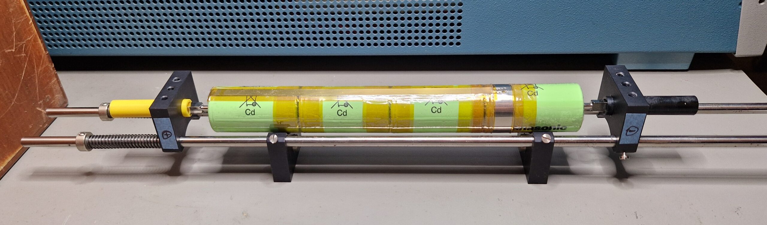
Isolated BNC inputs and DC supply input of the Tektronix THS 720Tektronix THS 720 battery compartment. The (+) electrode contact can be seen as a black square on the bottom left (around 7 o’clock)While powered on, the THS 700 Series oscilloscopes have quite a high current demand, which can be only supplied reliably by a Nickel-Cadmium (Ni-Cd) type of rechargeable batteries. Unfortunately, the Ni-Cd batteries have two disadvantages: they self-discharge over longer periods of time (at a rate of approx. 1% per day, it takes about 3 months for a complete discharge, inside of the scope they may discharge even faster within a couple of weeks) and they suffer to the memory effect (capacity deterioration due to charging/discharging cycles). I bought this oscilloscope for a very fair price (~200 EUR), however, with a dead Ni-Cd battery. The EEVblog users have investigated modern-era replacement possibilities such as NiMH batteries with special adapters which will fit inside of the oscilloscope battery compartment (length and diameter-wise). The alternative to this method is to buy certain Ni-Cd battery cells and combine them together into a battery pack.I was lucky to find an offer on Kleinanzeigen from a guy who already premade this kind of battery pack and I bought it from him for about ~50 EUR. This saved me a lot of time and tinkering because I didn’t have a spot welding machine in order to attach metal sheets to the electrode. So here is a comparison between the original THS 700 Series oscilloscope batteries and the DIY-type.
Comparison between THS7BAT and a DIY Ni-Cd battery packNi-Cd battery spot welding detail imageFour C-type cells (Panasonic Cadnica, model N-3000CR, Ni-Cd 1.2 V, 3000 mAh, Flat Top (non extending), diameter 26 mm, single cell length 50 mm, ~7 EUR/piece) were used and contacted in series and assembled with Kapton tape so they form a single battery unit. Unfortunately, the THS 720 oscilloscope demands the positive electrode (cathode) to be placed at a certain position along the battery axis – you can’t simply use the both ends of the batteries unless you want to modify your scope for this purpose. In order to meet the requirements, the positive battery electrode needs to be extended by spot-welding a thin metal sheet and connect it to a metal ring, located about 40 mm above the negative electrode (anode) of the bottom cell. The metal ring provides the positive battery supply connection to the oscilloscope. This is a very odd construction but that’s how the oscilloscope was made back in the mid 1990s. It’s important to notice that the metal sheets must be spot-welded to the battery electrodes in order to provide reliable electrical connections. Leads cannot be soldered to the battery electrodes directly for different reasons – if they come off, they can cause power loss or even shorts, the heat applied during soldering can also damage the battery cell. The metal sheet needs also to be sufficiently isolated with suitable non-conducting tape in order to prevent (potentially dangerous) battery shorts.
Ni-Cd battery cathode ring – detail image
Anyways, the Panasonic Cadnica replacement batteries turned out to work exceptionally well and provided enough power for a certain amount of time (depends on oscilloscope usage, perhaps 1 day with intermittent usage). I didn’t use the oscilloscope very much in the past and the battery was discharged as expected. In order to recharge the battery, I originally used the oscilloscope’s internal charging circuit, which “kinda” did the job. The charging at supplied voltage of 12 V and 1 A took around 24 hours. I noticed a significant heat-up of the battery packs up to ~45 °C, maybe 50 °C so I wasn’t quite sure about the unsupervised safety of this charging procedure. The max. charging temperature according to the datasheet is specified at +45 °C so I really hit the temperature limit. To avoid this in the future, I was looking for a fast Ni-Cd charger where I could quickly recharge the batteries without a significant heat build-up. There is a Tektronix THS7CHG Battery Charger on the 2nd hand market (e. g. eBay), however, it’s too rare and too expensive and not a viable option. An EEVblog user has constructed a similar charger with off-the-shelf components and 3D-printed housing. For a single Ni-Cd cell, the rapid charging time should be in the order of 1 … 2 hours at a nominal Voltage of 1.2 V and maximum currents of up to 4500 mA – compared to the 16-24 hours at standard charging currents (300 mA).
Robbe Power Peak Infinity 2 battery chargerRobbe charger, sitting on top of a switch-mode power supply during a charging operation
For this purpose, I bought a 2nd hand discontinued universal charger, which are very common in the fields of radio-controlled toys and RC models (drones, cars, boats etc.). It was manufactured by a German company called Robbe (type: Power Peak Infinity 2), which is capable of charging and discharging different types of batteries (NiMH, Lead Acid, Ni-Cd). In order to operate it, one needs a (switch-mode) power supply which provides the necessary voltages and currents for operation of the charger (e. g. 13.8 V and 0.1 … 5 A). The battery charger’s microcontroller monitors and regulates the output voltages and currents, which suits the charging profile of the batteries being recharged. In case of 4 Ni-Cd batteries, we need at least 4x 1.2 V = 4.8 V with a current limitation of 4.5 A (according to the Cadnica datasheet). The charging speed is limited by the battery temperature, the build-up of internal pressure and the so-called charge rate C. Typical charge rates are around 0.1 C while “fast” charge rates are around 0.5 C up to 1 C. Due to limitations of Ni-Cd batteries (memory effect, ~500 recharging cycles), they should be discharged first, then recharged at low rates (e. g. 0.1 C) to increase their longevity. For long-term storage of Ni-Cd batteries, Robbe user manual recommends to discharge them first and store them in a cold and dry place (e. g. in a fridge at 4 °C) in order to mitigate the performance deterioration due to the memory effect.
My experimental setup for battery charging and monitoring: Robbe charger, switch-mode power supply, Tektronix TDS 3034B oscilloscope with a P6139A probe and TCP202 current probe. In the center part of the image, the charging fixture for the Ni-Cd battery is shown. Not shown in picture: digital multimeter HP 34401A. Top left: Rubidium Precision Time Base (not used for this experiment, just casually laying around)Quick-and-dirty assembled Ni-Cd battery fixture from optics parts. The electrode contacts are just standard 4 mm banana plugs inserted into 4 mm banana couplings.
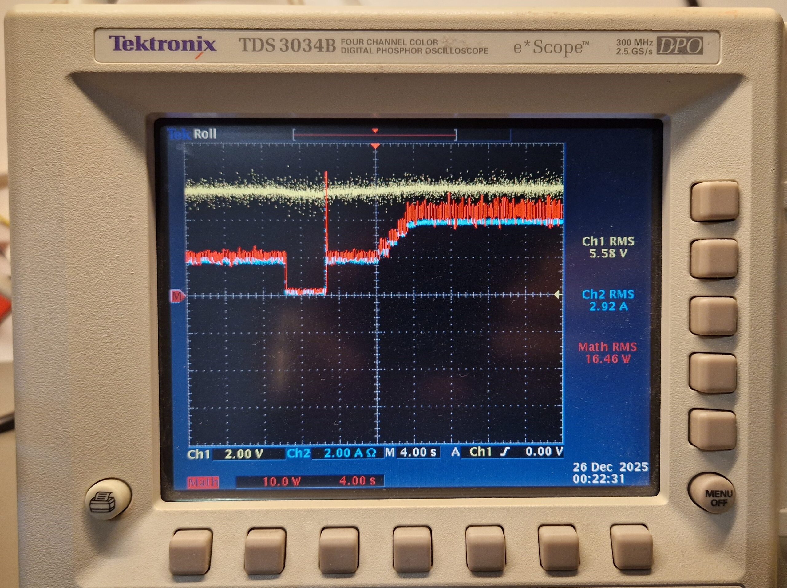
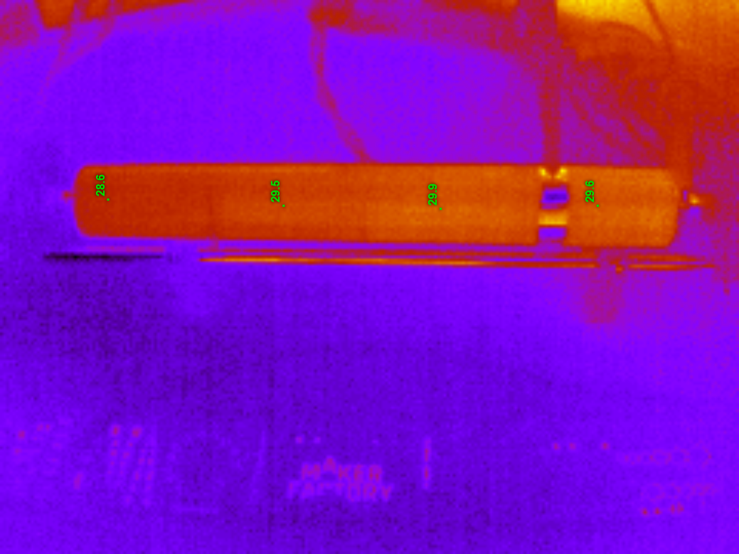
My charging/discharging setup looks as follows: the switch-mode power supply (JAMARA Germany DC Regulated Power Supply, Output: 13.8 V & 0-20 A) is connected to the charger. The charger output is then connected to the battery pack fixture. For my battery fixture, I used some spare optics parts I had at hand. The spring-loaded electrode helps to keep the battery in place and also helps to provide a reliable electrical contact. The recharger was powered on and set up to the “DISCHARGE -> CHARGE” mode, which is recommended by the Robbe manual. The battery under test had a remaining voltage of about 2.4 V and was discharged with a current of about 0.1 to 0.3 A. As soon as the battery was discharged to a certain threshold voltage (e. g. 1 V open circuit voltage), the charging cycle began by a slow ramp-up of the voltages and currents. After few minutes, the rapid charging is reached at approx. 6 V and 4.5 A (about 30 W), which corresponds to a charge rate of 1.5 C. I could observe some kind of a charge duty cycle, where the current flow stopped for a certain amount of time before continuing again – perhaps for thermal management purposes. The charging process took about 60 minutes, the estimated restored battery capacity (= transferred charge) was in the order of 3000 mAh. The temperature of the setup was monitored during the charging process with a thermal camera, however the battery pack didn’t heat up significantly in comparison to the mentioned THS 720 internal battery charger. The voltages were monitored by a digital multimeter HP 34401A and an oscilloscope Tektronix TDS 3064B, the current was monitored by a Tektronix TCP 202 current probe. This allowed me to estimate the power demand during the charging process.
Measured voltage of the empty Ni-Cd battery pack
Ongoing discharge, monitored via an oscilloscope
Charging ramp-up shortly after charging begins
Charging voltage, current and power at maximum output (6 V, 4.5 A)
Charging has finished
Thermal image (IR) of the experimental setup
Temperature measurement during Ni-Cd rapid charging
Thermal image of the battery setup, taken few minutes later
I was surprised how well and how fast this recharging process went. The DIY battery pack proved to be suitable alternative to the original battery pack Tektronix THS7BAT. Unfortunately, the Ni-Cd batteries age and need to be replaced over time. However, an inexpensive alternative with modern-day parts for a reasonable amount of money (~30 … 40 EUR) can be used to replace the original battery pack and extend the lifetime of the oscilloscope usage, at least until the internal electronic parts start to fail (e. g. the opto-couplers of this scope).
Tektronix THS 720, operational with a fresh recharged battery
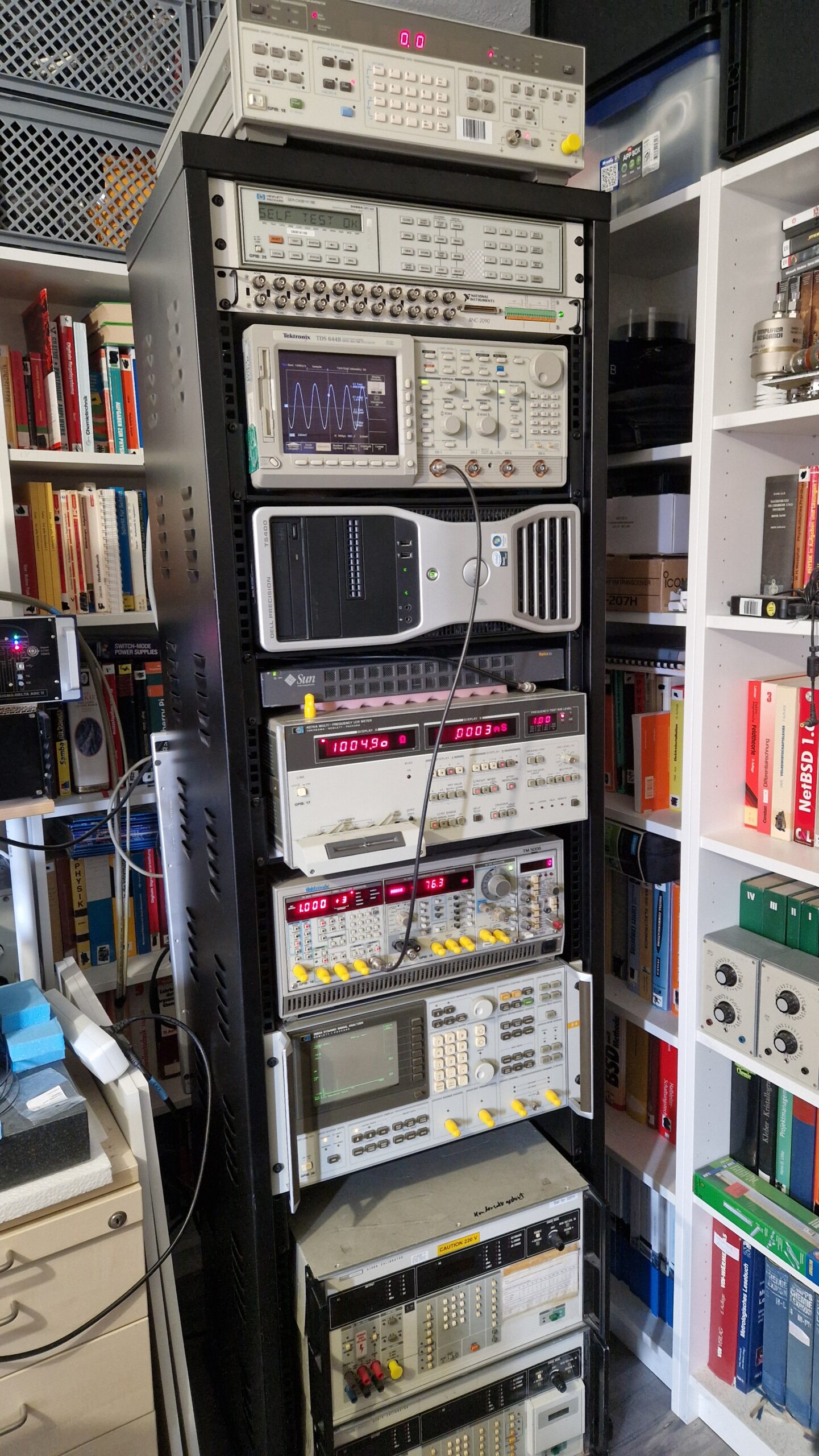
Yes, I have some kind of a Gear Acquisition Syndrome. Yes, I’m a Test Equipment Anonymous. Yes, I love Test Equipment! 🙂 However, this was bothering me for quite some time. The 19″ equipment was laying all over the place and I had some difficulties using it, since the instruments were bulky, scattered and there was no logical order as soon as I wanted to perform measurements. Luckily, a colleague of mine gave me a hint to buy a very cheap 19″ (42 HU) rack mount. This would solve few problems and also introduce new ones (more space for more equipment! Just kidding…). Anyways, I bought the rack mount and after few weeks of procrastinating, I finally equipped it with my 19″ sized test equipment. I’m pretty happy how it turned out. The most heavy parts are located at the bottom and lighter equipment is located at mid to top. It’s stable enough and won’t tip over and it can be easily moved around.
19″ Test Equipment rack mount.
Almost all instruments can be controlled remotely either via GPIB or RS232. An older Dell Workstation will be controlled via Windows Remote Desktop. Instruments from top to bottom are listed as follows:
HP 3325B – A 20 MHz frequency generator with some interesting features for audio testing
HP 3488A – Switch unit equipped with different modules. It’s used for automated, accurate and reliable signal switching or signal routing – it really depends on the used relay cards. I got few of them over the past years, e. g. types 44470A (10 CH multiplexer), 44471A (10 CH general-purpose relay module), 44472A (dual 4CH VHF switch module), 44473A (4×4 Matrix switch) and 44474A (16 bit digital I/O)
NI BNC-2090 is coupled with NI PCI-6110 (PCI multi-function-I/O-card with 4 analog inputs (12 bit, 5 MS/s per channel), 2x analog out, 8 digital I/O)
Tektronix TDS 644B, 4 CH, 500 MHz, 2 GS/s digital real-time oscilloscope. It’s a bit overkill for my audio-type applications – an excellent instrument for displaying waveforms, even RF stuff. A very useful feature is a GPIB interface for remote control and screenshot hardcopy (no need to use the disk drive)
Dell Precision T5400 workstation PC. It’s a 2007 era workstation which I bought probably around 2010 as a second hand PC. I used it like… forever. It was replaced by a faster workstation back in 2020. I haven’t dumped it because of the DVD burner and slots for 3x PCI and 3x PCIe cards. This makes it very valuable when it comes down to using data acquisition PCI cards from early to mid 2000’s era with a Win 7 or Win 10 operating system. Unfortunately this unit consumes a lot of power – it tends to heat up and it’s having thermal management difficulties during hot summers. Few of the ECC SD-RAMs failed over the past years but luckily they have been replaced easily. I tried to equip the three PCI slots with my oscilloscope cards, however, there were some serious thermal issues. I didn’t want to fry the cards so I put them inside of an external PCI expander system
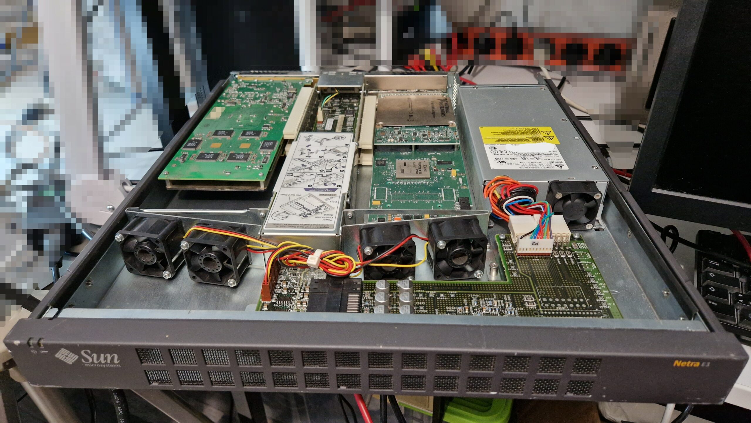
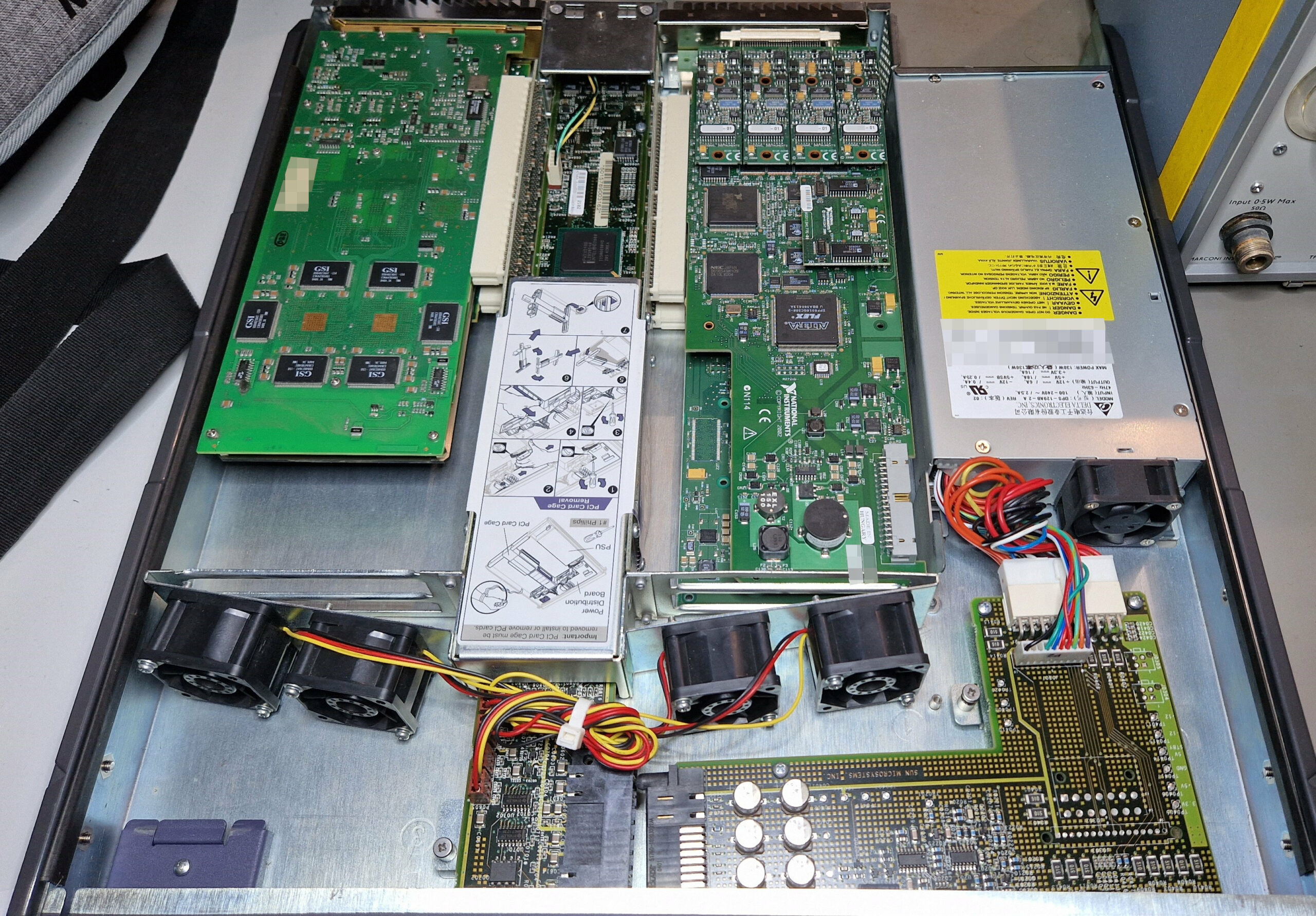
Sun Microsystems Netra E1. After having thermal issues and space problems inside of the Dell T5400, I was looking for a better solution to put the cards in a separate chassis and operate them via a PCIe/PCI bridge. Few solutions exist today, however only few are viable due to hardware/driver compatibility or power delivery constrains. The cheap expansion cards (mostly from China) can’t always deliver the 25-75 W of power to the oscilloscope card. In my case, as soon as the oscilloscope card demanded more power, the PC system crashed. After browsing eBay and looking for National Instruments’ “PXI-like” external chassis solution, I found Sun Microsystems’ Netra E1 as a viable option – however, the price was hefty. In retrospective, I’m glad I bought it because it was ready for use and it saved me a lot of time and trouble. The installation was super easy as PCI/PCIe bridge drivers exist at least since Windows XP. A downside of Netra E1 are the really loud fans. They work relentlessly at full speed; however, they keep the power-hungry cards at acceptable temperatures around 50-60 °C in comparison to 75-80 °C inside of Dell T5400!
Sun Microsystems Netra E1 – PCI Expansion System
Sun Microsystems Netra E1 – Top view.
Sun Microsystems Netra E1 – Back view.
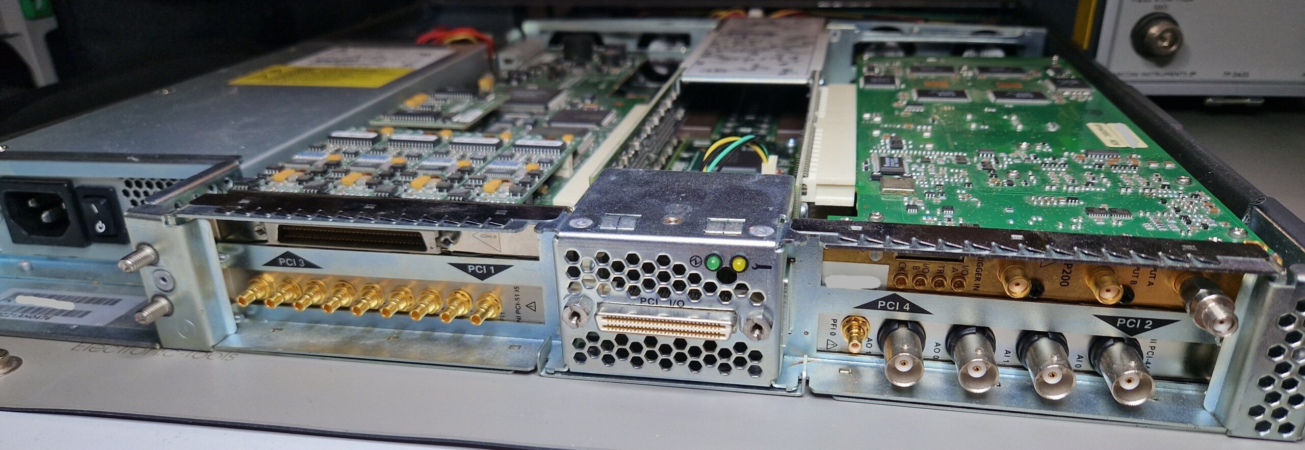
Unfortunately, Netra E1 is obsolete technology and no replacement parts exist on the 2nd hand market. Those units were produced around the year 2001 as an expansion system for Sun’s Netra Servers. I might be wrong about this but IIRC their PCI expansion product line was acquired by a company called MAGMA somewhere around mid 2000’s. MAGMA was specialized in building PCI Expander Systems for the Pro Tools Digital Audio Workstations (Pro Tools by Avid Technology, famous tor their audio/video editing software). eBay has some offers with MAGMA expansion chassis up to 16 PCI card slots, however they come at an unrealistic price of $500 to $1000, at least for a hobbyist budget. Anyways, beside the three existing PCI slots inside of the Dell workstation, I was able to put all of my four “power hungry” PCI cards (full length) inside of the 19″ chassis
NI PCI-6110: multi-function I/O card
NI PCI-5105: 8 channel, 12-bit, 60 MS/s digitizer/oscilloscope with up to 60 MHz analog bandwidth
NI PCI-4461: dynamic signal analyzer, basically a $10k sound card, still produced today – according to NI, it can be bought until 2024-12-31!
Agilent/Acqiris AP200: 1 channel, 500 MHz, 2 GS/s high-speed digitizer/averager card (used in radar tech or mass spectrometers)
Yokogawa/HP 4274A Multi-Frequency LCR Meter. I have a bunch of HP fixtures for components, unfortunately the LCR meter needs a repair. Should be hopefully an easy fix since the errors appear after warm-up. Fun fact: The Japanese government was very restrictive and protected their markets in the early days. In order to enter the Japanese market, companies from foreign countries such as United States were obliged to “team up” with a local Japanese manufacturer so they could sell their products in Japan. I guess HP teamed up with Yokogawa and Tektronix had a partnership with SONY. That’s the reason why there is occasionally a double company logo on some pieces of test equipment.
Tektronix TM5006 chassis equipped with
Tektronix FG5010, 20 MHz frequency generator (GPIB-controllable)
Tektronix AA 5001, audio analyzer capable of measuring Total Harmonic Distortion (THD), also GPIB-controllable
Tektronix SG505, audio frequency generator with exceptional ultra-low distortion sine-waves, perfect for audio amplifier testing
Tektronix DC 503, digital counter (doesn’t work, needs a repair)
HP 3562A Dynamic Signal Analyzer. A very capable FFT analyzer e. g. for audio and vibration testing and frequency response analysis in the µHz … 100 kHz regime
Fluke 5100B/5101B Calibrators. They can provide AC and DC voltages and currents and also resistances for calibration of up to 5.5 digit DMMs. Unfortunately, both need repair (power supply issues). Currently they are not in use – I’m hoping to repair them either later this year or maybe in early 2025
Surrounded by the rack mount are my book shelves with many books about physics, chemistry, operating systems and other stuff. A HPM 7177 digitizer can be seen at mid-left. There are only three cables left which are connected externally to the chassis: 230 V power, GPIB and Ethernet. I could replace GPIB with an NI GPIB-USB and Ethernet with WiFi. This would of course simplify the cable management but I’m very happy how everything turned out. I’ll need to find some lifting feet for the rack mount since it’s a bit overloaded with ~200 kg of equipment and it could cause damage the floor and the wheels over time.
Most of the test equipment seen here has been acquired during the past 3-4 years. Some pieces were really cheap (< 100 EUR), others rather expensive (> 300 EUR). It will be used for my laser interferometer and accelerometer calibration project which I plan to build in the future.
Tektronix TDS 3034B four channel color digital phosphor oscilloscope.
A “new” oscilloscope arrived in the lab just recently thanks to my friend Matt, who relayed the offer to me. It’s a wonderful instrument from the early 2000’s era: a Tektronix TDS 3034B Four Channel Color Digital Phosphor Oscilloscope. The oscilloscope’s analog bandwidth is specified at 300 MHz with a sample rate of 2.5 GS/s per each channel. It has a ton of options (e. g. FFT, 3LIM, 3TRG) and a communication module with VGA monitor output and GPIB/Ethernet/RS-232 for communication and control. There is also a battery compartment, however, the battery was not included. The “Waveform Intensity” knob simulates the intensity control of an analog oscilloscope with a cathode ray tube – therefore a “Digital Phosphor Oscilloscope” or DPO. The size of the oscilloscope is very convenient and perfect for a desk use – doesn’t take much space and it’s fast and responsive compared to my older Tektronix TDS 754D oscilloscope.
Tektronix TDS 3034B back side with battery/probe compartment.
I was able to set up the communication to my PC via GPIB (IEEE 488). Since I already had the Tektronix WaveStar Software for Oscilloscopes installed on my Windows 10 PC, I was able to quickly transfer screenshots/hardcopies, measurement data and sample data from the instrument to my PC. No diskettes or USB drives were needed. It is possible to control the oscilloscope remotely which is absolutely fantastic for measurement documentation and measurement automation purposes! It’s a great addition to the lab and it will serve to me as my daily workhorse among other oscilloscopes, of course.
Tektronix WaveStar for Oscilloscopes. Easy way to transfer screenshots and data from Tek TDS 3034B to a Windows PC.
Bandwidth Upgrade
It seems to be very common (even nowadays in 2024) that the oscilloscope manufacturers design a generic oscilloscope parts which can be used for different models. The oscilloscopes are then assembled with similar to identical hardware components (presumably because it’s cheaper manufacturing-wise) but the measurement capabilities are determined either by hardware (jumper settings) or by software (locked/unlocked options). For example, Rigol DHO 800/900 Series Oscilloscopes can be upgraded from 70 MHz to 100+ MHz via software. Thanks to Matt, he gave me a hint that the guys at EEVblog have figured out how to perform an upgrade of the Tektronix TDS Series oscilloscopes to different models. So already having an excellent 300 MHz & 2.5 GS/s oscilloscope at my fingertips, I was curious if I could upgrade it to the 3064B model which has 600 MHz analog bandwidth and 5 GS/s sample rate. I tried out the EEVblog’s upgrade procedure and it seemed to work without bricking the oscilloscope. I’ll just quickly summarize the procedure here.
*IDN? query via GPIB.
Tektronix TDS 3034B boot screen.
Boot up the device and set up the communication via GPIB (e. g. GPIB address and talker/listener mode). Connect the device to your GPIB controller
I used the National Instruments GPIB-USB-HS controller device along with current NI’s GPIB drivers (driver version doesn’t matter much, you could also use the VISA drivers from Keysight, Tektronix or Keithley). The TDS 3034B Firmware Version was v3.39
The communication between the PC and the oscilloscope was established with NI Measurement & Automation eXplorer’s (NI MAX) own GPIB Instrument Communication. I guess you could use any GPIB communication software, e. g. pyvisa for Python
Check whether the oscilloscope responds to the *IDN? query. If yes, proceed, if not – try to find the problem and fix it (obviously)
Send the following commands to the oscilloscope PASSWORD PITBULL MCONFIG TDS3064B
Just send (write) the commands in the order as shown above! Do not use a “GPIB query” since there will be no response action from the oscilloscope. Upper/lower case letters don’t matter.
Now power-cycle the oscilloscope (turn it off, wait few seconds and turn it on again). It should boot up with a new screen and new model. If it doesn’t show the new model, something went wrong with command transmission via GPIB. As far as I could tell, some models accept only different MCONFIG-commands, such as “MCONFIG TDS3054” without the letter “B” at the end. Anyways, after sending the commands via GPIB and power-cycling the oscilloscope, it should show up with the new model
Changing the TDS model will result in an uncompensated waveform. I observed a DC offset and noise on my CH1 through CH4 waveforms post-update. The solution to this problem is quite easy: wait some time (at least 10-15 minutes) for a warm-up and perform the Signal Path Compensation (SPC), which can be found in the Utility → System Config → Cal
menu. This will perform an internal calibration where the noise and offset errors are compensated. The oscilloscope should be ready for performing measurements afterwards
*IDN? query after BW upgrade.
Boot screen after BW upgrade.
Waveform pulse post-upgrade. Sample rate is at 5 GS/s.
Tek’s Signal Path Compensation.
That’s how it worked out for me. It took me just few minutes to convert a Tektronix TDS 3034B into a TDS 3064B. I’d recommend to check out the linked EEVblog thread for further information on the TDS 1000/2000/3000 Series upgrades. Of course I can’t be held responsible if you try it out and damage your instrument (e. g. calibration data or warranty is lost or the device is bricked) since I’m sharing this information and tried it out on my own oscilloscope. This is solely done at one’s own risk! Please be careful when trying out this procedure and please read the EEVblog thread prior to changing the instrument. Always make backups of your oscilloscope firmware prior to changes. Also hacking the device in order to use unlicensed software options is… well… “illegal”… I guess… Keysight’s Agents will hunt your PC down! 😉
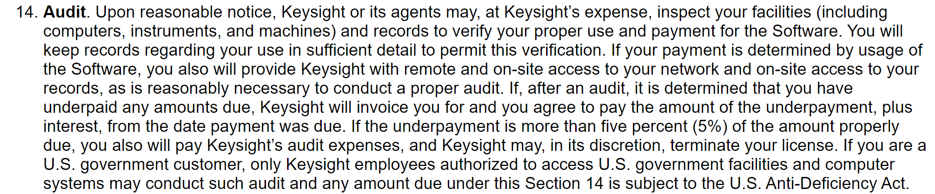
Excerpt taken from the Keysight N1500A EULA. This is not a joke (well, it’s a well-known meme), see it for yourself: https://helpfiles.keysight.com/csg/N1500A/License_Agreement.htm
Checking the Oscilloscope Analog Channel Bandwidth
I did some initial bandwidth testing with my Leo Bodnar Fast Risetime Pulse Generator. The pulser generates repetitive 10 MHz square waves (~1 Vpp) with a rise time of around (30 ± 2) ps. It can be used to easily test the oscilloscope’s analog channel input bandwidth. The analog bandwidth of an oscilloscope can be calculated as follows:
So a measured 10%-90% rise time of \(t_r = 1.000 ~\mathrm{ns}\) results in an analog bandwidth of \(0.35/(1.000 \cdot 10^{-9} ~\mathrm{s}) \approx 0.350 \cdot 10^9 ~\mathrm{Hz}\) or 0.35 GHz which is basically 350 MHz. So prior to the bandwidth upgrade we were expecting an oscilloscope bandwidth of ~300 MHz at a 2.5 GS/s sample rate, post-upgrade it should be around ~600 MHz and a 5 GS/s sample rate. I’ve measured the rise time of all four channels in order to see if there are any significant differences between them. The oscilloscope settings were as follows: Coupling: DC, Termination: 50 Ω, Trigger: External, Acquisition Mode: 64× average per acquisition at 10k points and 5.00 GS/s. The trigger was delayed by approx. -10 ns.
Tektronix TDS 3034B CH1 risetime.
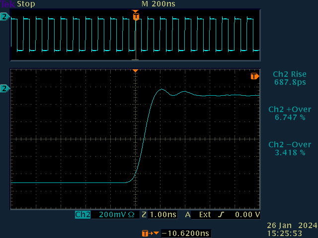
Tektronix TDS 3064B CH1 risetime.
Tektronix TDS 3034B CH2 risetime.
Tektronix TDS 3064B CH2 risetime.
Tektronix TDS 3034B CH3 risetime.
Tektronix TDS 3064B CH3 risetime.
Tektronix TDS 3034B CH4 risetime.
Tektronix TDS 3064B CH4 risetime.
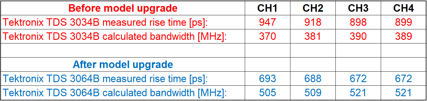
The measurement results are summarized in the table below.
Analog bandwidth calculations from measured rise times for each oscilloscope channel. Comparison between Tektronix TDS 3034B before model upgrade and after model upgrade to TDS 3064B.
As we can see, the full bandwidth of 600 MHz for a Tektronix TDS 3064B has not been achieved. However, there is a measurable improvement. Channels 3 and 4 seem to have a slightly higher bandwidth than channels 1 and 2. The rise time measurements deviate on each acquisition so I would estimate an uncertainty in the rise time measurements of approx. ±10 ps. I also wonder if the overshoot/undershoot calculations are correct. I’ll have to look into this manually, since the data samples can be exported in a CSV file.
Conclusion
Nevertheless, the bandwidth upgrade was successful! 500 MHz analog bandwidth at 5 GS/s is more than enough for my needs before stepping into the GHz time domain regime. And no need for a battery if there is a food compartment in your oscilloscope! Tested successfully with carrots! 😉
A spectrum analyzer (SA) is a very useful tool when it comes to measure spectra of radio frequency signals. I recently acquired a 2004 era spectrum analyzer. It’s from a Japanese test equipment manufacturer Anritsu and the model number is MS2661N. Luckily there are operating manuals available online but I wasn’t able to find service manuals for this type of spectrum analyzer on the internet. There are some service manuals available for similar models of spectrum analyzers (e. g. MS2650/MS2660) which would allow troubleshooting but I would be lost if the instrument breaks.
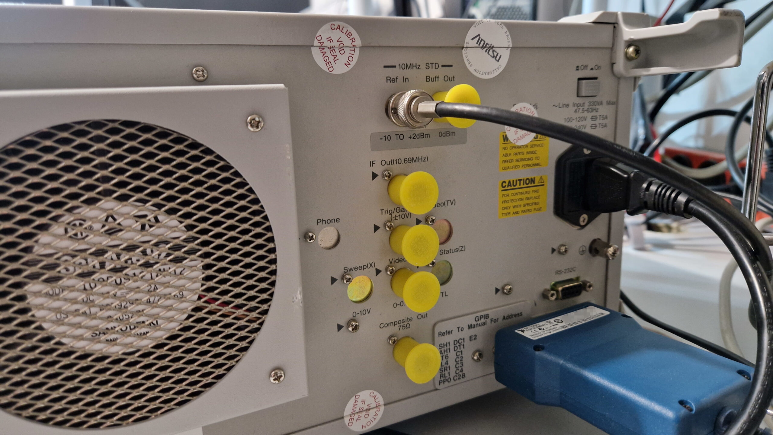
Anritsu MS2661N Spectrum Analyzer (100 Hz – 3 GHz). Those blue handles totally aren’t butchered from Rohde & Schwarz test equipment… Sacrilege! Don’t ask!
However, I’ve been looking for a decent SA for a longer time and stumbled upon the Anritsu MS2661N. It had a bunch of very nice and useful features: frequency range 100 Hz to 3 GHz, 30 Hz resolution and video bandwidth, oven controlled crystal oscillator (OCXO), GPIB interface, 10 MHz reference IN/OUT and a tracking generator ranging from 9 kHz to 3 GHz. I was looking for a similar SA from HP/Agilent 8590 Series or Tektronix but there were no attractive offers at the time. Either the SA frequency range was too low for modern ages (1 GHz) or outside of my measurement capabilities (26 GHz), the price was either too high or it was partially broken. There were also 75 Ohm spectrum analyzers which aren’t very useful for what I’m doing. On the other side, the documentation for HP/Tek hardware is the real deal so leaving this kind of test equipment ecosystems was a tough decision.
Long story short: I wasn’t disappointed and the SA works perfectly fine. I don’t want to write a lengthily blog about it. One of the first experiments was connecting my GPS disciplined oscillator to the signal generator and spectrum analyzer simultaneously in order to provide the same external reference for both instruments and checking if the frequency (1.5 GHz) and the amplitude (-35 dBm) are accurate. Acquiring measurements was super easy and the operation of the SA is very straight-forward.
Agilent E4432B Signal Generator. Note that the EXT REF is on and the output signal is referenced to a 10 MHz GPS disciplined oscillator.
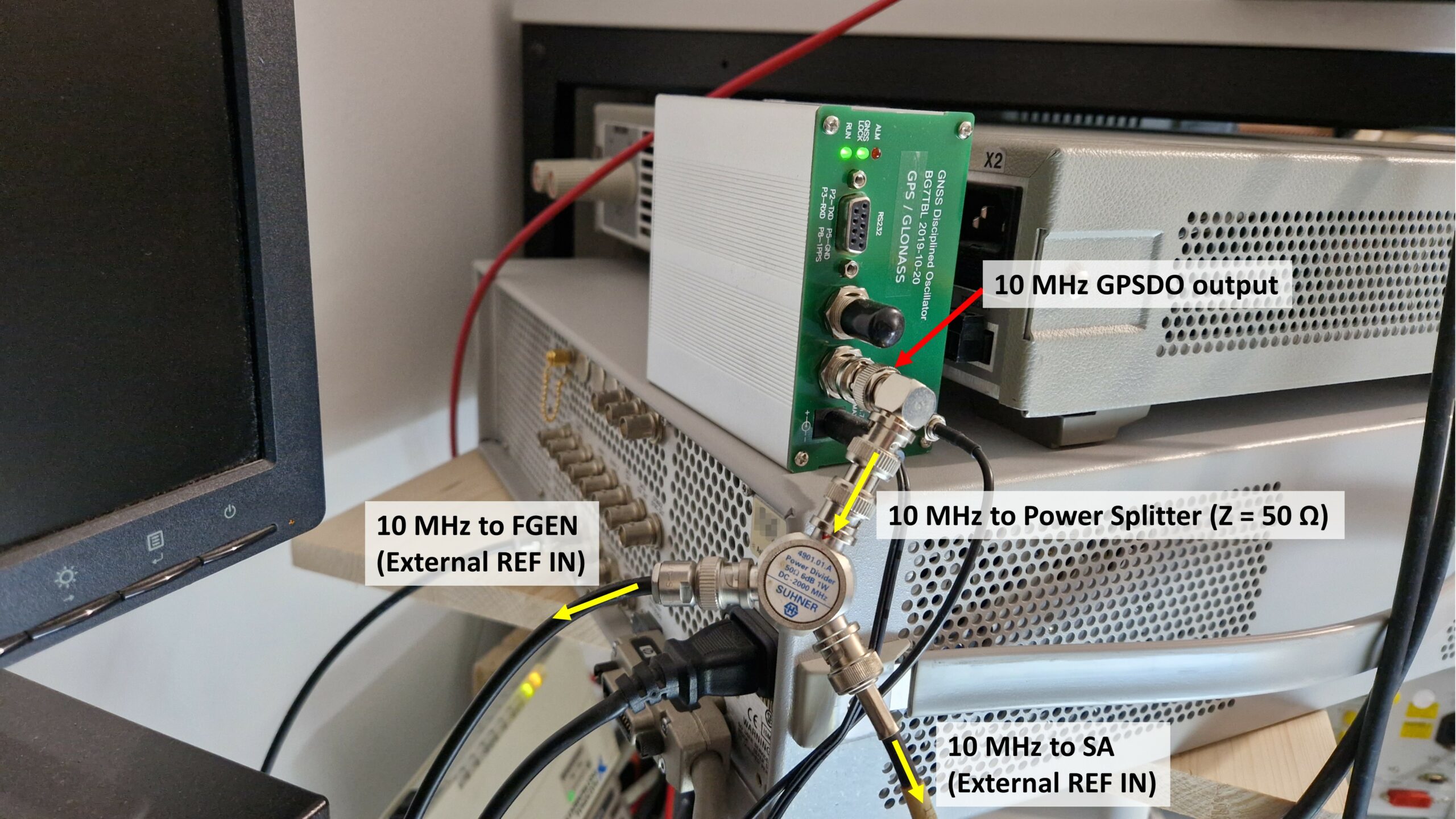
10 MHz reference signal distribution from a GPS Disciplined Oscillator (GPSDO).
Back side of the Anritsu MS2661N. The 10 MHz signal is fed into the REF IN.
Documentation of Measurements
I would consider the somewhat cumbersome recording of readings as a minor disadvantage of this SA. Taking a photograph of the display may be “quick and dirty” but you have to deal with bad image quality due to reflections, visible RGB pixels and picture alignment. It is possible to take screenshots in bitmap format (BMP) but one needs a special type of a Memory Card (basically a PCMCIA or PC Card) in order to save the screenshots on an external storage. That’s really unfortunate but measuring instruments of that era were either equipped by a floppy disk or Memory Carc. I was always afraid of damaging the fragile pins while pushing the PCMCIA card in its slot although it is rated for 10k mating cycles. The MS2661N type SA even has a 75 Ohm composite out – it’s possible to record video stills in the NTSC format. However, there are two elegant methods which I would like to show how to transfer the readout from the instrument to the personal computer (PC) by modern means.
A photograph taken of the frequency spectrum. The image shows LCD pixels, scratches on the surface of the front panel and reflections due to bad light conditions.
Method 1: Sending a Hard Copy from SA to a PC
Back in the days, the measurement results such as frequency spectra would be printed on a piece of paper as a part of the documentation. A device called printer or plotter was needed and the process was called “hard copy”. The difference between a printer and plotter is how the drawing is generated: while the printer generates text and images line by line, a plotter can draw vectors in a X-Y-coordinate system. HP developed its own printer control language back in 1977 for this purpose – the HP-GL or Hewlett-Packard Graphics Language. HP-GL consists of a set of commands like PU (pen up), PD (pen down), PAxx,yy (plot absoute) and PRxx,yy (plot relative) in order to control a plotter, which is basically an electro-mechanically actuated pen. The commands are transmitted in plain ASCII via GPIB or RS-232C interfaces. If we were somehow able to capture the HP-GL ASCII code, it should be possible to generate a lossless vector graphics instead of a lossy bitmap.
An example of the acquired HP-GL code in a text editor.
Hardware Requirements
Besides the already mentioned spectrum analyzer one needs either a GPIB/USB or GPIB/Ethernet adapter. I have tested it successfully with a National Instruments GPIB-ENET/100 on a Windows 10 machine with NI 488.2 v17.6 drivers. It should also work with a NI GPIB-USB-HS+ (Chinese clone) adapter.
Software Requirements
I was looking for a quick solution how to acquire hard copies. Thanks to einball on a certain Discord channel 😉 for showing me the KE5FX 7470.EXE HP-GL/2 Plotter Emulator. John Miles, KE5FX, already wrote a software back in 2001 which does emulate a HP 7470A pen plotter. The 7470.EXE is still maintained by John and supports popular spectrum analyzers from HP and Tektronix. His software is able to fetch the HP-GL ASCII via GPIB and render the hard copy image on the screen. The image may be saved in a bitmap format (BMP, TIFF, GIF) or in a vector format (PLT, HGL). I have tested John’s software with Anritsu MS2661N and it worked perfectly fine. I suppose this could work on similar Anritsu spectrum analyzer models, such as MS2661C.
Setting up the Spectrum Analyzer
Here is a brief summary how to obtain a hard copy from an Anritsu MS2661N spectrum analyzer:
Connect the spectrum analyzer to the GPIB adapter and boot up the device
Go to the Interface menu and use settings as followed → GPIB My Address: 1, Connect to Controller: NONE, Connect to Prt/Plt: GPIB, Connect to Peripheral: NONE
The SA wants to send its data via GPIB to a plotter. It’s important to disable the “Connect to Controller” option, otherwise it won’t be possible to select GPIB as “Connect to Prt/Plt”. The GPIB address is set arbitrarily to 1
Go to Copy Cont menu (Page 1) → Select Plotter
Copy Cont menu (Page 2) → Plotter Setup → Select following options: HP-GL, Paper Size: A4 Full Size, Location: Auto, Item: All, Plotter Address: 2
It’s important to set the “Plotter Address” value to a different number than the “GPIB My Address“. If both addresses share the same number, the hard copy will result in a timeout error
Install John’s 7470.EXE software and start the HP 7470A Emulator. There is no need to change the settings of the GPIB controller, it works out of the box. Click on GPIB → Plotter addressable at 2. The selected address in 7470.EXE should be identical as the previously set Plotter Address. In order to obtain a hard copy, press the button w and the 7470.EXE should display a message like shown in the screenshot below. Once you press the Copy button on the spectrum analyzer, a data transfer progress should be visible. It takes about 10-15 seconds to transfer the data (approx 7-10 kb) from the SA to the PC. Once it’s complete, an image of the current frequency spectrum is shown on the display. That’s it.
HP7470A Plotter Emulator in “Reading data from instrument” mode (Button: “w”)
The downloaded hard copy in KE5FX’s plotter emulator software 7470.EXE
Creating Publication-Quality Vector Images
At this point, it’s possible to save the acquired hard copy in a bitmap image format. If one needs a publication quality images – which should be free of compression artifacts – one should save the images in a vector format such as PLT/HPGL. This workflow proved to be a little bit inconvenient but it’s perfectly doable. Save the hard copy as .PLT and open the image in a HP-GL supported viewer. John suggests few of them on his website – I’ve tried CERN’s HP-GL viewer. It’s distributed free of charge and still maintained by the developers. Download their viewer and load the PLT-image. If the colors seem wrong, there is a setting where you can change the pen colors. Once done, it’s possible to export the PLT image as PostScript (PS) or Encapsulated PostScript (EPS) or print as PDF. EPS files can be embedded in LaTeX documents or can be imported in a vector graphics editor such as Inkscape.
This hard copy was exported into EPS format and loaded in Inkscape. It’s possible to further edit the image (create annotations etc.)
CERN’s HP-GL Viewer may further process the PLT vector image and export it in different formats such as PS/EPS/PDF
The results turned out to be really good. Especially the vector images are crisp and sharp. One can zoom in without any image quality losses. The printouts on my laser printer are perfect. A little downside would be few breaks in the workflow: one has to use three different applications in order to obtain, convert and process the images. But it’s worth it 😉
Method 2: Readout Data via pyvisa and Plot it via Matplotlib
A different method to plot the frequency spectra would be by downloading the acquired raw data via GPIB and plot it directly. This is exactly what I’ve done. I’ll share the Python code down below. It’s possible to refine the plot by automating more stuff: one can generate annotations directly from queried instrument settings. Just put enough time in it and you’ll get superb results. The plotted image can be saved directly in a Scalable Vector Graphics (SVG) or any supported bitmap/compressed format.
Spectrum analyzer data plotted via Python’s library Matplotlib
# -*- coding: utf-8 -*-
"""
Created on Tue Jan 3 16:45:39 2023
@author: DH7DN
"""
import numpy as np
import pyvisa
import pandas as pd
import matplotlib.pyplot as plt
#%% Open the pyvisa Resource Manager
rm = pyvisa.ResourceManager()
print(rm.list_resources())
#%% Create the Spectrum Analyzer object for Anritsu MS2661N at GPIB address 13
sa = rm.open_resource('GPIB0::13::INSTR')
# Print the *IDN? query
print(sa.query('*IDN?'))
#%% Take a measurement
# Set frequency mode to CENTER-SPAN
sa.write('FRQ 0')
# Set the center frequency in Hz
cf = 1.5E9
sa.write('CF ' + str(cf) + ' HZ')
# Set span in Hz
span = 10000
sa.write('SP ' + str(span) + ' HZ')
# Take a frequency sweep (TS)
sa.write('TS')
# Select ASCII DATA with 'BIN 0' according to Programming Manual
print(sa.write('BIN 0'))
# Create a Python pandas Series
data = pd.Series([], dtype=object)
# Fetch data, convert string to float, print the power level values
for i in np.arange(501):
data[i] = float(sa.query('XMA? ' + str(i) + ',1')) * 0.01
print(data[i])
#%% Plot the results
# Generate the frequency values for the x-axis
f = np.linspace(cf-span/2, cf+span/2, 501)
# Plot the results, set a title and label the axes
plt.plot(f, data)
plt.xlabel('f in Hz')
plt.ylabel('Power Level in dBm')
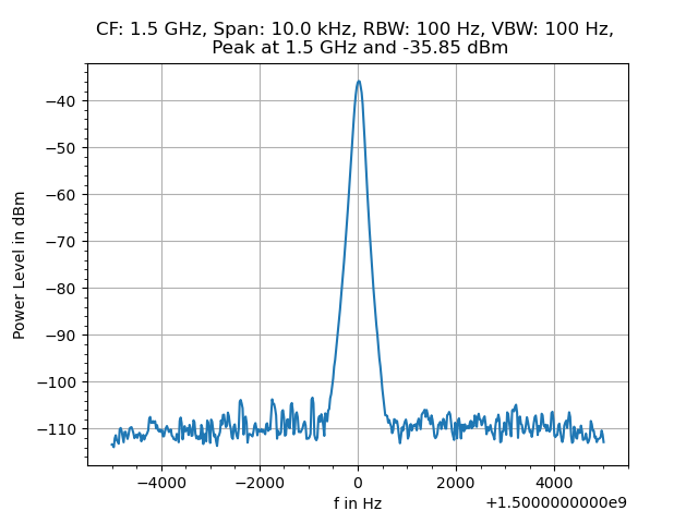
plt.title('CF: 1.5 GHz, Span: 10.0 kHz, RBW: 100 Hz, VBW: 100 Hz, \n Peak at 1.5 GHz and -35.85 dBm')
plt.grid(axis='both')
plt.minorticks_on()
plt.show()
Few things to consider when using Python to obtain data from the spectrum analyzer:
Anritsu MS2661N acquires only 501 data points per sweep
The frequency axis values need to be generated manually. I used numpy‘s linspace method. It was a bit tricky because you one has to change the generation of frequency step values depending on whether parameters “Center Frequency & Span” or “Start/Stop Frequency” are used
Fetching the data takes quite some time (approx. 30 seconds). This is due to the fact that every single data point needs to be queried with the XMA? command in a for-loop. This is at least how it’s done in an example from Anritsu’s Programming Manual. I haven’t figured out yet how to fetch a block of data
Summary and Conclusion
I was clearly impressed how easy it was to obtain good quality frequency spectra images from a 20 year old instrument. I’ll refine the workflows and do further testing in Python. It should be possible to do all of this “automagically” via one little Python script. So far I’m really happy with the results where I don’t have to rely on smartphone pictures anymore. Thanks to einball for his help (basically googling for me) and to John (KE5FX) for writing his plotter emulator which helped me a lot to obtain hard copies from my SA. That’s it for today! Happy measurements! 😉
Today’s modern technology is full of sensors. Sensing temperature, motion, force, humidity, sound, electricity, radiation – basically every imaginable physical quantity – necessary to measure and understand our environment. This is usually done with so-called transducers (sometimes abbreviated as Xducers) which convert the measured physical quantity (e. g. temperature or any kind of a signal) into a different physical quantity (e. g. resistance, voltage) or any other type of signal. In many cases, the transducer converts the measured physical quantity into an electrical signal which is used as an input to a digital voltmeter or an analog-to-digital converter. The conversion into electrical quantities is highly practical in order to be able to connect the transducer with our measurement instruments or our microcontrollers (which are basically small computers). A special kind of transducers I want to talk about here today are piezoelectric accelerometers.
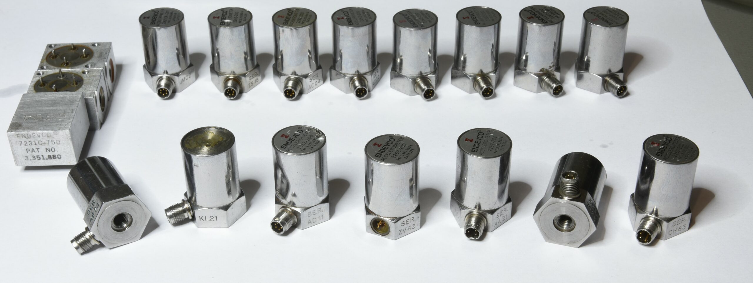
Figure 1: Small selection of newly acquired accelerometers. The accelerometers in the front row are obviously damaged and will not be tested/calibrated. The accelerometers in the back row have no visible defects although they may have some issues. The previous owner labeled them as “replaced due to repair”. Whether they work or not has to be determined.
Just recently I’ve acquired a huge batch of piezoelectric accelerometers in an unknown condition which need to be tested for functionality. The goal of this project is to develop a small prototype calibration device in order to be able to calibrate piezoelectric accelerometers by comparison method.
Piezoelectric Accelerometers
Working Principle
Piezoelectric (PE) accelerometers are basically “acceleration-to-charge” transducers. They rely on the piezoelectric effect which – in simple words – converts mechanical energy into electrical energy. A piezoelectric transducer consists of a piezoelectric material (e. g. quartz, lithium niobate) and a small seismic mass.
Figure 2: Elements of a single-ended compression-type piezoelectric accelerometer, presumably from manufacturer Endevco (Model 213E, 233, 2272 or similar). The accelerometer housing was cut open in order to see the seismic mass, piezoelectric disks and electric connections.
As soon as dynamic forces act on the spring-mass-system along the acceleration-sensitive axis, mechanical stress is introduced on the piezoelectric material which is mounted inside of the accelerometer housing (see Figure 2). The resulting deformation of the PE material causes a polarization which in return generates a change in surface charge density. The change in surface charge density is directly proportional to the mechanical stresses (e. g. force or pressure) and therefore proportional to the acting force or acceleration (if you remember the Newton’s 2nd law \( F = ma \longrightarrow a = F/m \)). The resulting change in surface charge density can be detected, amplified and converted into a measurable voltage with a proper signal conditioner or so-called “charge amplifier”. For simplicity’s sake I’ll refer to “charges generated by the accelerometer” instead of “polarization and change in surface charge density of the PE material”.
Harmonic Oscillator
From a mechanics point of view, the basic construction of a PE accelerometer can be approximated as a spring-mass-system with a low dampening as shown in Figure 3.
Figure 3: Analogy of a piezoelectric accelerometer to a harmonic oscillator.
The harmonic oscillator is a very basic physical model of a spring-mass-dampener system. The huge advantage of this model is its simplicity: the harmonic oscillator equations contain the Newton’s laws of motion (\(F = ma\)) and Hooke’s law (\(F = kx\)) which can be solved analytically using so-called differential equations. While I’m skipping the mathematics part here and just want to mention that in reality things are more complex, some of the results of the differential equation for a driven harmonic oscillator are shown in Figure 3. Applying oscillations on a spring-mass-dampener system leads to the curves (Bode plots) showed in Figure 3. One of critical parameters of a harmonic oscillator is the natural frequency \(\omega_\mathrm{n}\). It’s a particular frequency where the spring-mass-system is oscillated (or “shaken”) in resonance, e. g. the mechanical system responses with very large displacement amplitudes while being excited by very small amplitudes. Resonance phenomena can be experienced in everyday situations like music instruments, swinging bridges, vibrations in cars driving at certain speeds, tuning forks etc.
For example, sinusoidal excitations of an accelerometer at its resonance frequency can lead to damage or change of its specified properties, e. g. sensitivity. A high resonance frequency is achieved by using stiff material (spring constant \(k\) should be high) and small seismic mass. In case of an accelerometer, the resonance frequency should be as high as possible, usually in the order of 30…50 kHz for high-frequency or shock measurements. Brüel & Kjaer suggests in [1] that the typical useable frequency range of an accelerometer is specified to approx 30% of the natural frequency.
The equation \( \omega_\mathrm{n} = \sqrt{k/m} \) for the undamped natural frequency suggests that using no seismic mass would lead theoretically to an infinite natural frequency! In reality, we need a small seismic mass – it has to be just big enough so it can compress or tension our spring (which is basically the PE material) through its inertia. We need to create mechanical stresses on the PE material in order to generate our precious charges. Basically a larger seismic mass leads to a larger signal output which is exploited in the low-frequency range (\(f \ll 10 ~ \mathrm{Hz}\)) and in seismometers.
Measuring Accelerations with a PE Accelerometer
The amounts of charge generated by an PE accelerometer are very minuscule. In order to get a measureable amount of charge, the PE elements are stacked in parallel as seen in Fig. 1. We’re talking about tens to hundreds of femto-Coulombs (fC) per m/s² of acceleration up to few pico-Coulombs (or pC) per m/s². Typical values are in the order of few pC where \(1~\mathrm{pC} = 10^{-12}~\mathrm{A} \cdot \mathrm{s}\). Just imagine charging a small capacitor with a capacitance of C = 100 pF and a voltage of U = 0.1 V and you will get according to the capacitor equation \(Q = C \cdot U\) a value of \(Q = 10~\mathrm{pC}\). High-intensity accelerations in the order of 1 … 100 km/s² – which are found in crash or shock testing – may generate few nano-Coulombs of charge. Measuring such minuscule quantities requires a somewhat specialized test equipment: ultra low noise coaxial cables with limited length and a signal conditioner for impedance matching, signal amplification and filtering.
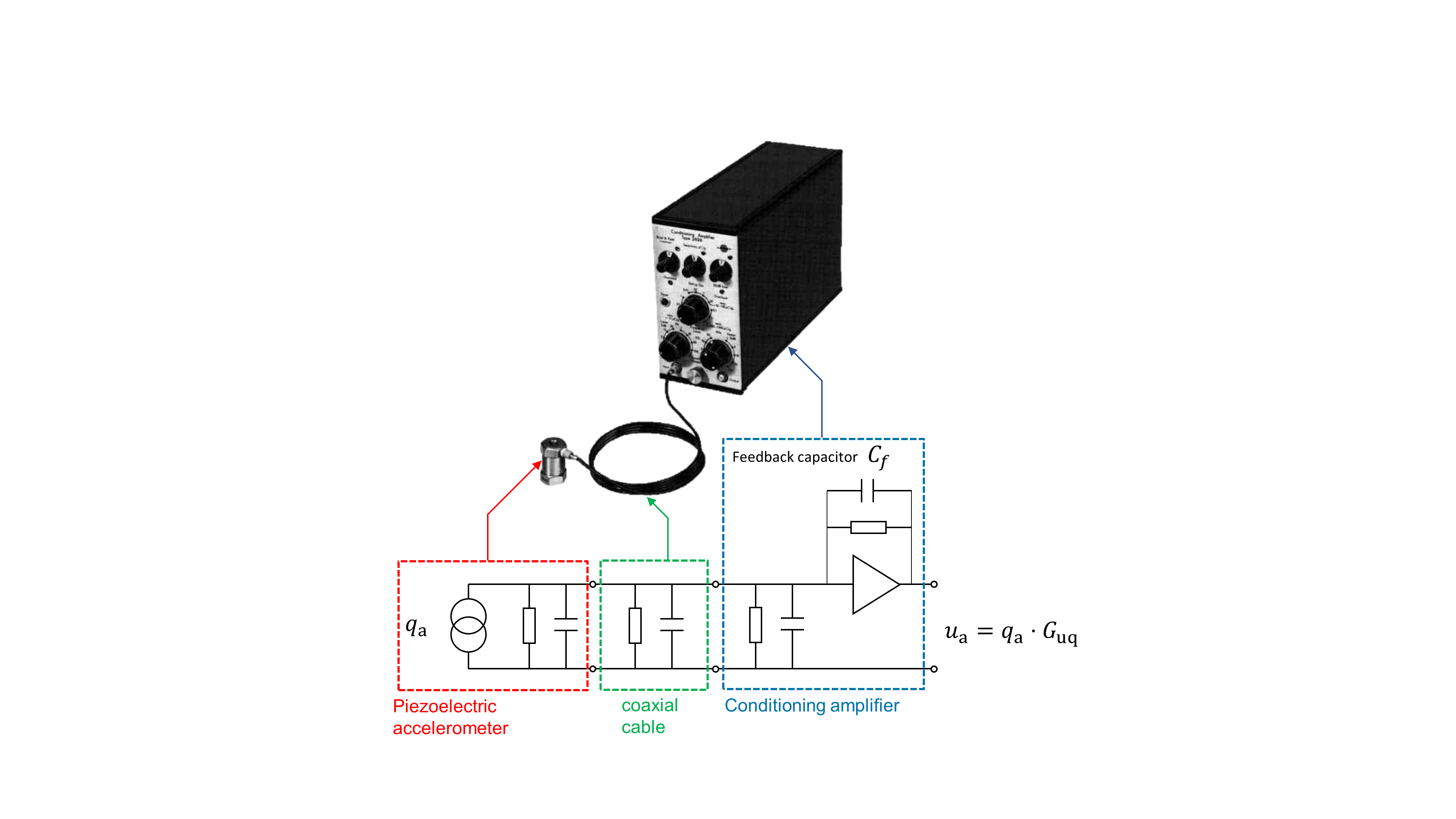
Figure 4: Measurement setup consisting of a PE accelerometer (Brüel & Kjaer 8305), coaxial cable (Brüel & Kjaer AO0038) and a conditioning amplifier (Brüel & Kjaer 2525) and its equivalent circuit diagram. The PE accelerometer can be described as a charge source. The PE element acts as a capacitor in parallel with a very high internal leakage resistance. Images taken from [1].The use of PE accelerometers is pretty much straight-forward. The accelerometer needs to be attached to a vibration source which can be virtually anything: electric motor, mountain bike, structure of a bridge, washing machine, car armature, rocket engine etc. In order to perform vibration measurements properly, one has to consider many experimental issues such as mounting, temperature influences, cable fixture, grounding loops, amplifier settings and few more. Informations on this topic can be gathered from instruction manuals and application notes from different manufacturers. In order to perform accurate measurements, the instruments needs to be calibrated.
Calibration of a Piezoelectric Accelerometer
As soon as one buys (very expensive) acceleration measurement equipment, the new instruments will be factory calibrated and the manufacturer will provide calibration certificates to the customer. A calibration certificate contains important information how to establish the relationship between the input quantity (acceleration) and the output quantity (charge or voltage). This information is usually called sensitivity of an accelerometer. The sensitivity of an accelerometer is determined during a process called calibration. According to JCGM:200 (2012), the International Vocabulary in Metrology (VIM), a calibration is
[…] operation that, under specified conditions, in a first step, establishes a relation between the quantity values with measurement uncertainties provided by measurement standards and corresponding indications with associated measurement uncertainties and, in a second step, uses this information to establish a relation for obtaining a measurement result from an indication.
In other words: a calibration is a comparison between input and output quantities of any kind. The input quantity is provided by a well-known standard, the output quantity is provided by a device under test (DUT). In case of an PE accelerometer, the input quantity is an acceleration, the output quantity is charge (or voltage if using a conditioning amplifier).
Unfortunately – when buying surplus stuff – there is always a risk of getting either a defective or incomplete unit. The provided calibration certificates may be either wrong or got lost. Some PE accelerometers are well over 50 years old and may have drifted over time. For my purposes, I’ll have to skip the “measurement uncertainties” part for now because I want to test the accelerometers for their qualitative condition and functionality. I’ll return to the metrology part in a future project.
Description of the Calibration
The calibration process is shown in a block diagram (Figure 5). In order to generate an acceleration \(a(t)\), we need to set our Accelerometer Standard (REF) and the Device Under Test (DUT) in an oscillating motion. This is usually done with an electrodynamic exciter – a technical term for “shaker” or “loudspeaker”. The working principle of an electrodynamic exciter is identical to the principle of the well-known loudspeaker. We’re generating a low distortion sinusoidal signal with a function generator which is fed into a power amplifier. The amplified signal drives the coil of the moving part inside of the exciter which in return creates the oscillating motion. Amplitude and frequency of acceleration are set by the function generator, which are typically in the range from 10 Hz to 10 kHz and 1 m/s² to 200 m/s². The frequency and amplitude ranges depend strongly on the construction of the electrodynamic shaker and the total weight of the DUT and REF accelerometers.
Figure 5: Experimental setup (block diagram) for back-to-back calibration of a piezoelectric accelerometer. The comparison method according to ISO 16063-21 is described in [2] and [3].The generated motion is applied to both accelerometers, which are physically connected to each other. In this case, the DUT is mounted or screwed on the REF accelerometer in so-called back-to-back or piggy-back configuration. Our goal is now to establish the relationship between the input and output quantities by calculating the acceleration and measuring the output voltage of the DUT measuring chain. Basically, the charge sensitivity \( S_\mathrm{qa,DUT} \) of the DUT can be calculated as follows:
The shown equation might look scary and complicated but it’s pretty straightforward: we’re measuring the output voltages of both measuring chains and multiplying their ratio with the charge sensitivity of our reference accelerometer (\(S_\mathrm{qa,REF}\)). Afterwards we’re multiplying the resulting expression with the ratio of transfer functions of our charge amplifiers (\(G_\mathrm{uq}\)), which have to be determined by a different type of calibration. For the sake of completeness, I would like to mention that the sensitivities and transfer functions in general are complex values (e. g. \( \underline{S}_\mathrm{qa} = |S_\mathrm{qa}| \cdot \exp{(\mathrm{j}\omega t + \varphi_\mathrm{qa}}) \)) and we’re dealing with the magnitude \( |S_\mathrm{qa}| \) of the complex transfer function. I’ll try to cover this in a future blog post.
Experimental Setup
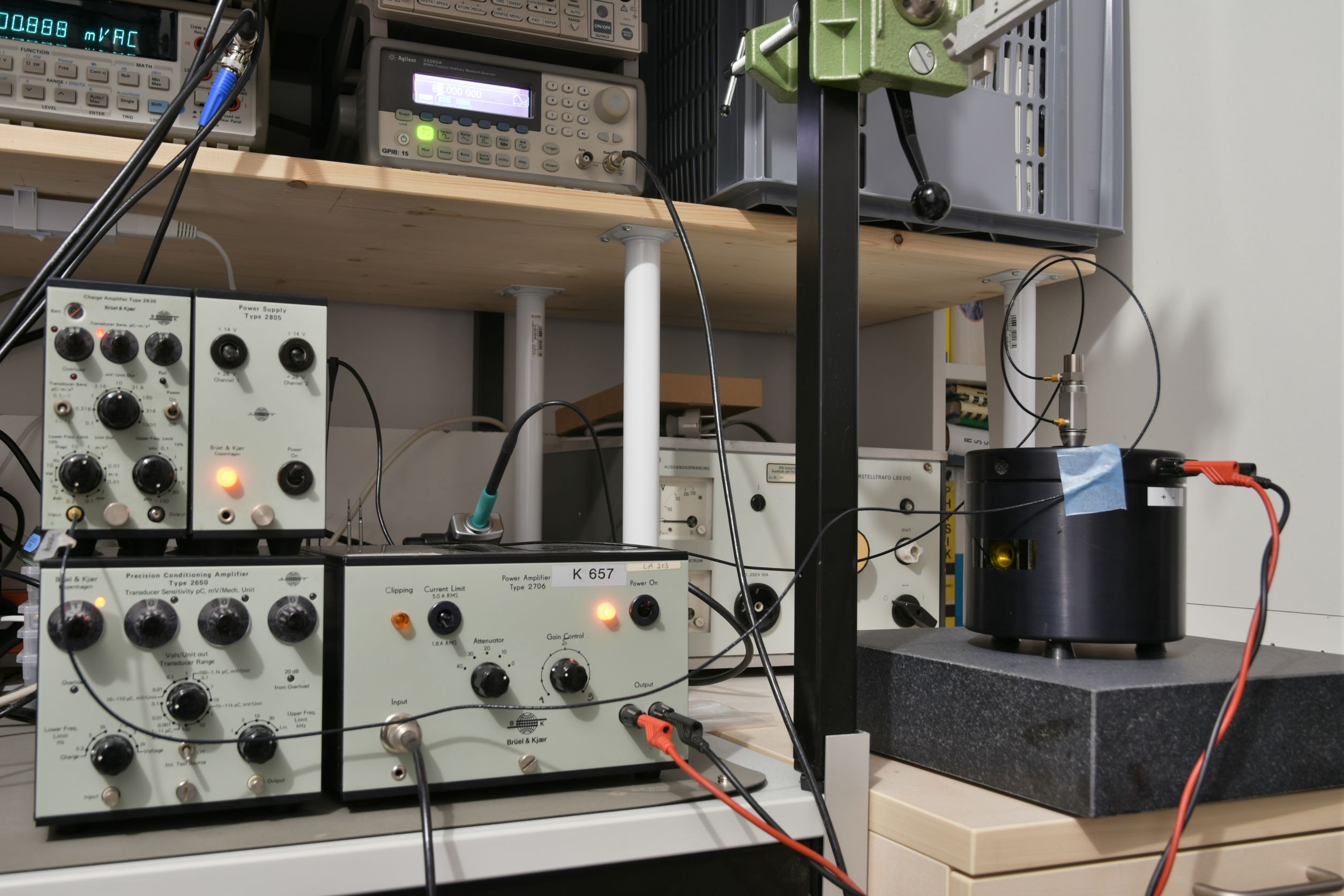
Since we need to perform the measurements over a wide set of frequencies, it is highly recommended to automate the task as much as possible. The instrument control, data acquisition and data analysis can be done with a PC. I’m using Python 3.9 with pyvisa, pandas and numpy on a Windows 10 machine. My accelerometer reference standard is a Kistler 8076K piezoelectric back-to-back type accelerometer. For the purpose of this experiment, I’ve tested two different PE accelerometers: Brüel & Kjaer 4371 and Endevco 2276, which are so-called “single-ended” accelerometers. Single-ended type accelerometers can be mounted on the top of a back-to-back type accelerometer and therefore calibrated by comparison method. The vibrations are generated by a Brüel & Kjaer 4809 electrodynamic exciter which is connected to a Brüel & Kjaer Type 2706 Power Amplifier and an Agilent 33250A frequency generator. I’ve used two charge amplifiers for the accelerometers, basically Brüel & Kjaer Types 2650 (REF) and 2635 (DUT). They were connected to HP 34401A digital multimeters. AC voltage measurements were performed in “ACV mode” which outputs the root mean square (RMS) voltage of the respective measurement chain signal output. An oscilloscope can be used to monitor the output waveforms in order to detect unwanted noise and distortions. This is a small downside of RMS measurements: the DC offsets and noise fully contribute to the measurement result.
Back-to-back calibration setup. The Device Under Test (Brüel & Kjaer 4371) can be seen mounted on the top while the Reference Accelerometer (Kistler 8076K) is “sandwiched” between the DUT and the electrodynamic exciter.
Experimental setup used for acceleration calibration by comparison. The electrodynamic exciter (Brüel & Kjaer 4809, right hand side) carries the DUT and REF in the back-to-back configuration. The exciter is connected to a power amplifier (Brüel & Kjaer 2706, lower mid).
Brüel & Kjaer charge amplifiers. Left: Type 2650, mid: Type 2635, right: Power supply Type 2805.
Typical low noise cables used for piezoelectric transducer calibration. Endevco 3090C can be seen on the left hand side. Brüel & Kjaer AO0038-D012 is shown on the right hand side. Both cables have a miniature 10-32 UNF coaxial connectors, also known as Microdot.
Setting up the devices wasn’t very difficult. The electrodynamic exciter needs a stable and massive base along with an adequate vibration isolation. If the vibration isolation is neglected, the vibrations are coupled into the desk and into the building. Using hard foam between the desk and granite block proved being very inexpensive and efficient. The support for low noise cables are also improvised. The cable mounting is a major source of experimental errors. Due to the triboelectric effect, a bending or vibrating coaxial cable also generates charges which are superimposing the measured accelerometer signal. In short words: the reference accelerometer is measuring a slightly higher acceleration than expected. Therefore the sensitivity drops due to \( S = q/a\). This can be seen in the measurement results at frequencies below 25 Hz. At higher frequencies (e. g. > 25 Hz) the displacement amplitude of the vibration becomes very small and the triboelectric effect becomes negligible. I’ve used a torque wrench with 2.0 Nm and the contact surfaces were slightly lubricated in order to prevent deviations at higher frequencies (>5 kHz).
Measurement Results
Figure 6: Frequency response (magnitude) of Endevco 2276 piezoelectric accelerometer in comparison with datasheet specifications.
The calibration result can be seen on the left hand side in Figure 6. The top curve represents the charge sensitivity of the DUT plotted vs. excitation frequency. There are some deviations in the frequency response which are really annoying but I’m really satisfied with the overall result. Calculations of the relative deviation of the charge sensitivity at a reference frequency of 160 Hz can be compared with the data provided by the manufacturer. A 5% deviation at 6 kHz is in a good agreement with the specifications! My measurements show even higher deviations at frequencies f > 6 kHz so there must be some kind of systematic error which has to be investigated. Nevertheless, the measurement is automated and it takes approx. 5 minutes for a “sweep” of 31 discrete frequencies in the range from 10 Hz to 10 kHz. I’ve used standardized frequencies which are known as Third Octave Series according to ISO 266. The bottom graph shows the acceleration amplitude over the frequency range. I’m ramping up slowly in order to minimize distortions. A limit of 20 m/s² is set for noise reasons in my apartment – the generated sine tones can be very annoying and I don’t want to wear ear protection all the time.
Summary and Conclusion
HP 3562A Dynamic Signal Analyzer can be used to perform FFT measurements.
FFT analysis and total harmonic distortion measurement performed on a HP 3562A dynamic signal analyzer.
Excerpt of the Python code used for automating the calibration procedure.
Oscilloscope screenshot showing sinusoidal signals and measured parameters such as RMS amplitude and phase shift between Channel 1 (REF) and Channel 2 (DUT).
This project clearly is a success! It took much time and effort in order to get the experiments straight and to automate the measurements. I was able to perform a calibration of a piezoelectric accelerometer with decent quality equipment. The results are “not bad” although I see much room for future improvements. I’ll have to improve the measuring chains and eliminate noise sources. I’d like to improve the Python code and generate a Graphical User Interface (GUI) for calibration purposes. Playing with a HP 3562A Dynamic Signal Analyzer was also very fun! I was able to dump the FFT measurement data (Thanks to Delrin for his Python hint!) via GPIB and didn’t rely on photographs of the display. A little downside of this instrument is its loudness and electricity consumption in the order of 400 W. I’ll certainly use the signal snalyzer during the winter months in order to heat my apartment 😉 I’m literally scratching on the surface in the fields of vibration measurements and the future will bring more interesting projects. The ultimate goal is to build a laser interferometer as an acceleration reference standard and to estimate the uncertainties of the built calibration devices.
References
[1] Serridge and Licht, Piezoelectric Accelerometer and Vibration Preamplifier Handbook, Brüel & Kjaer Naerum, Denmark, 1987
[2] Methods for the calibration of vibration and shock transducers – Part 21: Vibration calibration by comparison to a reference transducer, ISO 16063-21:2003
[3] Richtlinie DKD-R 3-1, Blatt 3 Kalibrierung von Beschleunigungsmessgeräten nach dem Vergleichsverfahren – Sinus- und Multisinus-Anregung, Ausgabe 05/2020, Revision 0, Physikalisch-Technische Bundesanstalt, Braunschweig und Berlin. DOI: 10.7795/550.20200527