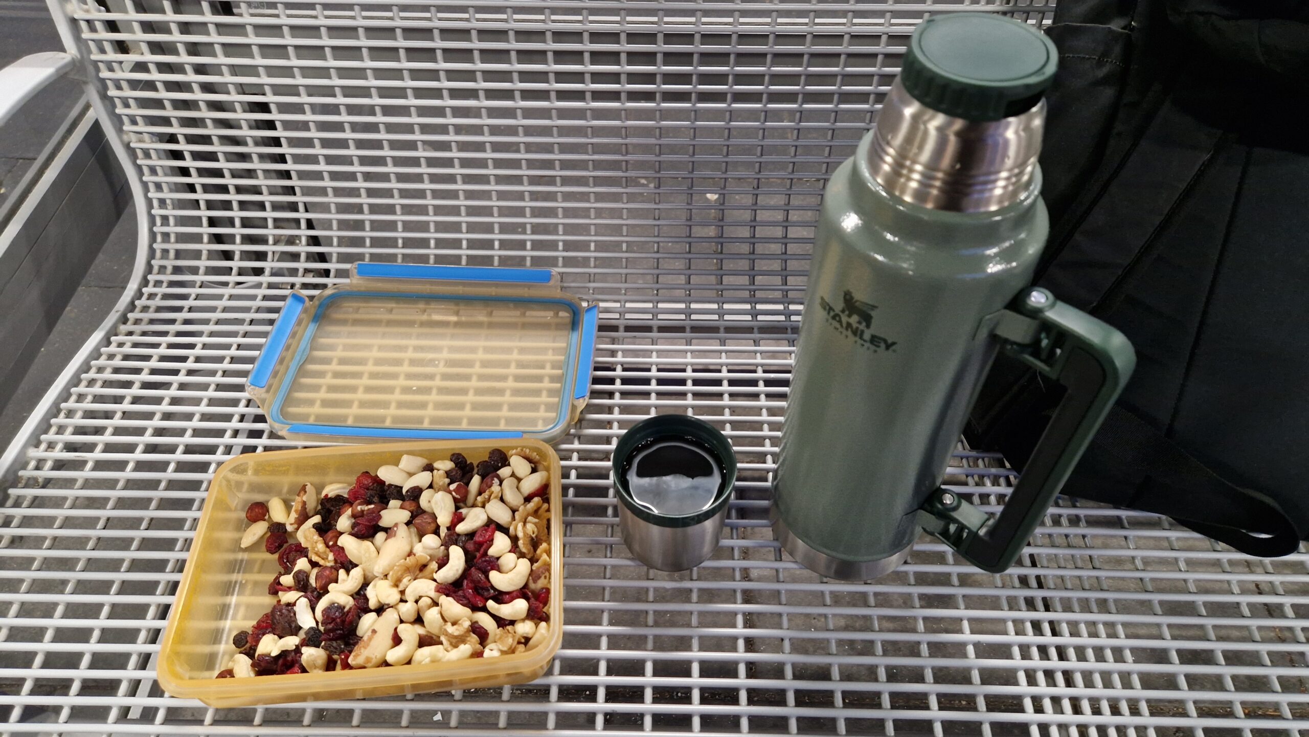
Coffee, nuts and berries! Everything a happy brain needs…
Happy New Year 2026 everyone! I hope you celebrated the new year’s holidays in peace with your families and friends. I’ve had some coffee and nuts, FeelsGoodMan!
As always, the year ahead looks ambitious. I plan to keep writing about my electronics projects, test equipment, precision measurements, and the tools that make all of this possible.
I’ve also noticed that I’m having troubles with writing blog articles for different reasons. One of my ongoing challenges is streamlining the writing process itself: keeping track of measurements, photos, schematics, revisions, and all the little iterative steps that never quite fit neatly into a finished article. Improving that workflow is a project of its own — but one that should make future posts clearer and more consistent. I also plan to use some “AI” or LLM-generated assistance text in order to overcome some “typically human” things like procrastination or writer’s blocks. This won’t compromise the integrity of my blog, because I don’t trust the current LLMs. There is currently no way around the scientific method or good scientific practices when it comes down to writing somewhat serious technical articles. Because this blog is mostly an “one-man-project”, I’m still dependent on your feedback as a reader. Please leave me an email if you find errors in my articles so I can correct them properly.
Unfortunately, I am always very busy and have little time for hobby projects. Time remains the most limited resource. Between work, projects, and everyday life, writing detailed technical articles is slow, but the intention for 2026 is very much to publish more than in 2025 — even if progress happens one careful step at a time. I’m aiming for 5…7 articles per year, depending on the topic and complexity of the article.
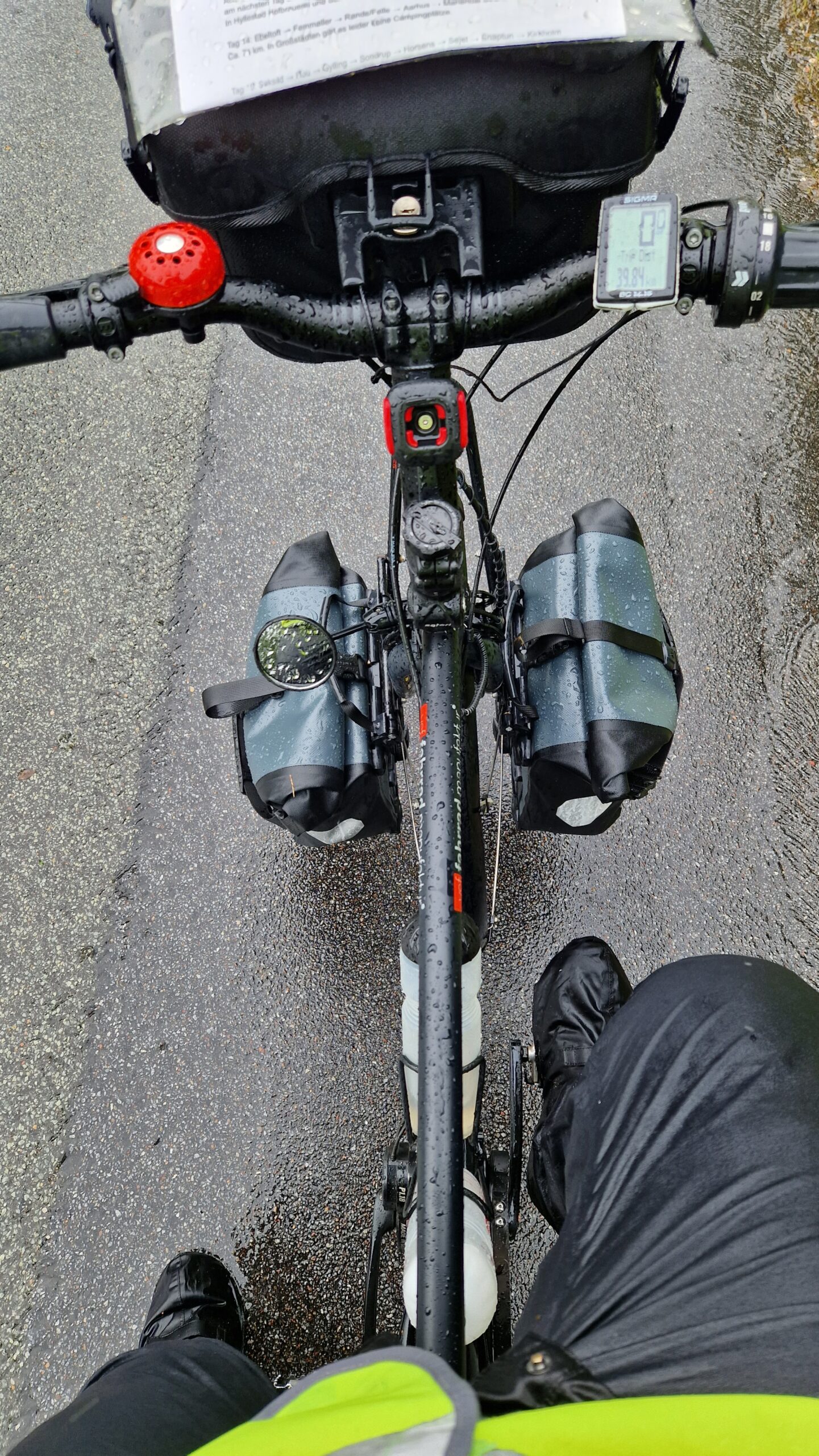
Outside of the lab, 2026 also comes with a bigger adventure: my second trip to Norway, continuing last year’s bike route from Bergen towards North. Long-distance bikepacking, combined with outdoor activities, camping, minimalism and self-sufficiency, fits perfectly with the spirit of this blog. I’m looking forward to sharing my travel impressions and lessons learned from the road.
Thank you for reading, experimenting, measuring, and building alongside me. May your probes be well compensated, your measurements stable, your antennas erected (in the best possible way) — and your projects successful in 2026.
Merry day after Christmas everyone! I hope everyone is having a good time and doing fun projects during holidays and vacation. I’m trying to write a blog post again, so today’s blog entry will be about some of my efforts to recharge a battery! Can’t be that hard, can it?
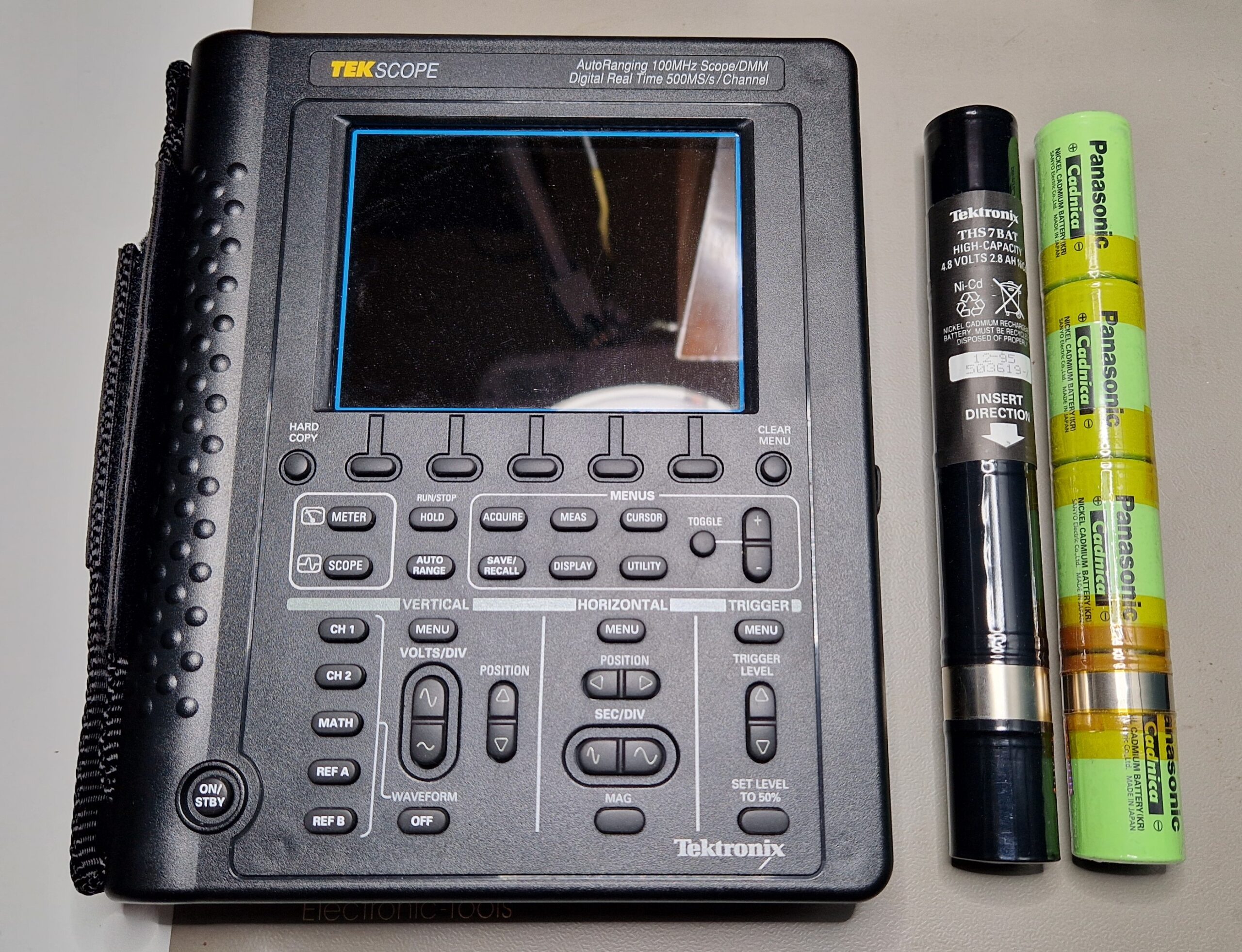
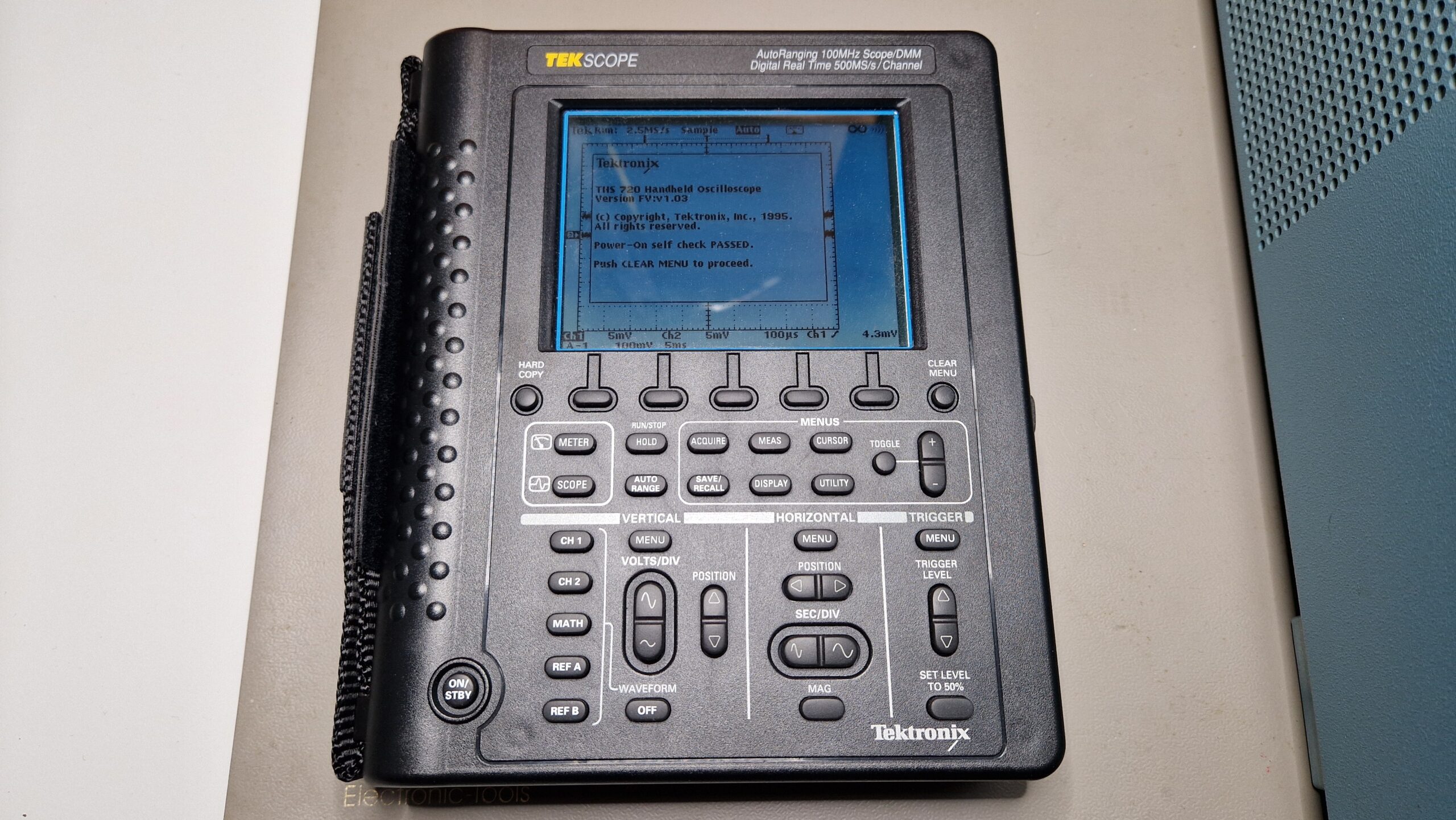
Tektronix THS 720 with rechargeable batteries. The original battery pack is labeled THS7BAT.
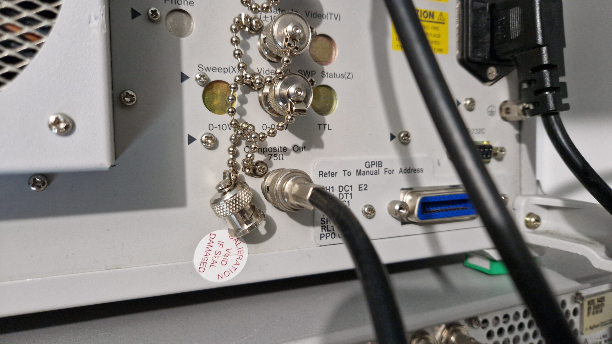
The Tektronix THS 720 is a portable and battery-operated 2 channel 100 MHz analog bandwidth, 500 MS/s oscilloscope with isolated BNC inputs and an integrated digital multimeter (DMM). It is a very useful tool for troubleshooting electronics or servicing (switch-mode) power supplies due to its isolated input channels. It can perform “floating” measurements and measure voltage differences safely on arbitrary potentials (similar to a handheld DMM). When testing switch-mode power supplies (SMPS, having a galvanic isolation and line voltages, e. g. 230 V) with an “ordinary” oscilloscope, keep in mind that the probe ground connector (GND) provides a direct and low impedance path to the oscilloscope chassis (mains earth referenced). This is potentially very dangerous, because if you connect your GND to a “floating” Device Under Test (DUT) at a higher voltage potential, the GND connector creates an electrical short between the DUT and the oscilloscope chassis. If the DUT and chassis are somehow connected through protective earth (PE), it can short out line voltages directly via your oscilloscope and perhaps ruin your day, too (danger of being electrocuted). In order to avoid these electrical safety dangers, the serviced DUT needs to be powered through an isolation transformer as a safety measure – or alternatively – it has to be probed by either using a high-voltage differential probe (for example Tektronix P5205A) or via a battery-powered, isolated (“floating”) oscilloscope (e. g. Tektronix THS 700 Series or Fluke ScopeMeter). There is an excellent explanation video on this matter from Dave Jones of EEVblog on YouTube.
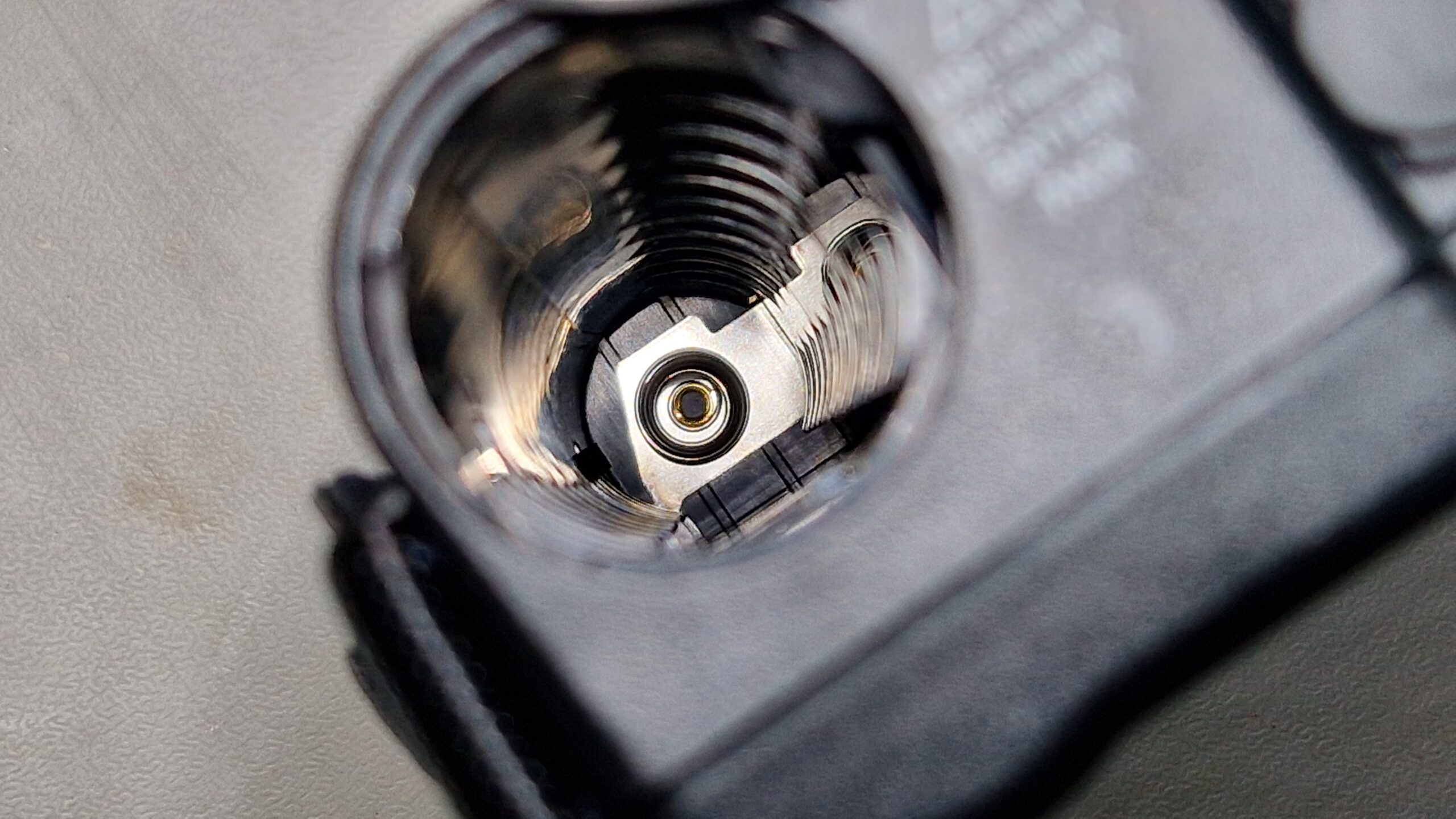
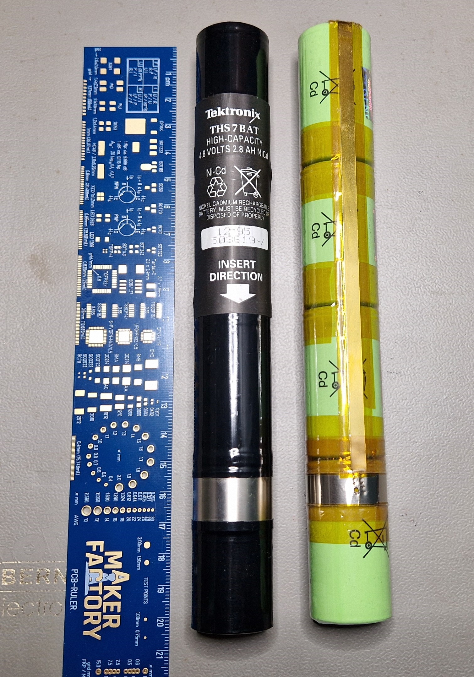
Isolated BNC inputs and DC supply input of the Tektronix THS 720Tektronix THS 720 battery compartment. The (+) electrode contact can be seen as a black square on the bottom left (around 7 o’clock)While powered on, the THS 700 Series oscilloscopes have quite a high current demand, which can be only supplied reliably by a Nickel-Cadmium (Ni-Cd) type of rechargeable batteries. Unfortunately, the Ni-Cd batteries have two disadvantages: they self-discharge over longer periods of time (at a rate of approx. 1% per day, it takes about 3 months for a complete discharge, inside of the scope they may discharge even faster within a couple of weeks) and they suffer to the memory effect (capacity deterioration due to charging/discharging cycles). I bought this oscilloscope for a very fair price (~200 EUR), however, with a dead Ni-Cd battery. The EEVblog users have investigated modern-era replacement possibilities such as NiMH batteries with special adapters which will fit inside of the oscilloscope battery compartment (length and diameter-wise). The alternative to this method is to buy certain Ni-Cd battery cells and combine them together into a battery pack.I was lucky to find an offer on Kleinanzeigen from a guy who already premade this kind of battery pack and I bought it from him for about ~50 EUR. This saved me a lot of time and tinkering because I didn’t have a spot welding machine in order to attach metal sheets to the electrode. So here is a comparison between the original THS 700 Series oscilloscope batteries and the DIY-type.
Comparison between THS7BAT and a DIY Ni-Cd battery packNi-Cd battery spot welding detail imageFour C-type cells (Panasonic Cadnica, model N-3000CR, Ni-Cd 1.2 V, 3000 mAh, Flat Top (non extending), diameter 26 mm, single cell length 50 mm, ~7 EUR/piece) were used and contacted in series and assembled with Kapton tape so they form a single battery unit. Unfortunately, the THS 720 oscilloscope demands the positive electrode (cathode) to be placed at a certain position along the battery axis – you can’t simply use the both ends of the batteries unless you want to modify your scope for this purpose. In order to meet the requirements, the positive battery electrode needs to be extended by spot-welding a thin metal sheet and connect it to a metal ring, located about 40 mm above the negative electrode (anode) of the bottom cell. The metal ring provides the positive battery supply connection to the oscilloscope. This is a very odd construction but that’s how the oscilloscope was made back in the mid 1990s. It’s important to notice that the metal sheets must be spot-welded to the battery electrodes in order to provide reliable electrical connections. Leads cannot be soldered to the battery electrodes directly for different reasons – if they come off, they can cause power loss or even shorts, the heat applied during soldering can also damage the battery cell. The metal sheet needs also to be sufficiently isolated with suitable non-conducting tape in order to prevent (potentially dangerous) battery shorts.
Ni-Cd battery cathode ring – detail image
Anyways, the Panasonic Cadnica replacement batteries turned out to work exceptionally well and provided enough power for a certain amount of time (depends on oscilloscope usage, perhaps 1 day with intermittent usage). I didn’t use the oscilloscope very much in the past and the battery was discharged as expected. In order to recharge the battery, I originally used the oscilloscope’s internal charging circuit, which “kinda” did the job. The charging at supplied voltage of 12 V and 1 A took around 24 hours. I noticed a significant heat-up of the battery packs up to ~45 °C, maybe 50 °C so I wasn’t quite sure about the unsupervised safety of this charging procedure. The max. charging temperature according to the datasheet is specified at +45 °C so I really hit the temperature limit. To avoid this in the future, I was looking for a fast Ni-Cd charger where I could quickly recharge the batteries without a significant heat build-up. There is a Tektronix THS7CHG Battery Charger on the 2nd hand market (e. g. eBay), however, it’s too rare and too expensive and not a viable option. An EEVblog user has constructed a similar charger with off-the-shelf components and 3D-printed housing. For a single Ni-Cd cell, the rapid charging time should be in the order of 1 … 2 hours at a nominal Voltage of 1.2 V and maximum currents of up to 4500 mA – compared to the 16-24 hours at standard charging currents (300 mA).
Robbe Power Peak Infinity 2 battery chargerRobbe charger, sitting on top of a switch-mode power supply during a charging operation
For this purpose, I bought a 2nd hand discontinued universal charger, which are very common in the fields of radio-controlled toys and RC models (drones, cars, boats etc.). It was manufactured by a German company called Robbe (type: Power Peak Infinity 2), which is capable of charging and discharging different types of batteries (NiMH, Lead Acid, Ni-Cd). In order to operate it, one needs a (switch-mode) power supply which provides the necessary voltages and currents for operation of the charger (e. g. 13.8 V and 0.1 … 5 A). The battery charger’s microcontroller monitors and regulates the output voltages and currents, which suits the charging profile of the batteries being recharged. In case of 4 Ni-Cd batteries, we need at least 4x 1.2 V = 4.8 V with a current limitation of 4.5 A (according to the Cadnica datasheet). The charging speed is limited by the battery temperature, the build-up of internal pressure and the so-called charge rate C. Typical charge rates are around 0.1 C while “fast” charge rates are around 0.5 C up to 1 C. Due to limitations of Ni-Cd batteries (memory effect, ~500 recharging cycles), they should be discharged first, then recharged at low rates (e. g. 0.1 C) to increase their longevity. For long-term storage of Ni-Cd batteries, Robbe user manual recommends to discharge them first and store them in a cold and dry place (e. g. in a fridge at 4 °C) in order to mitigate the performance deterioration due to the memory effect.
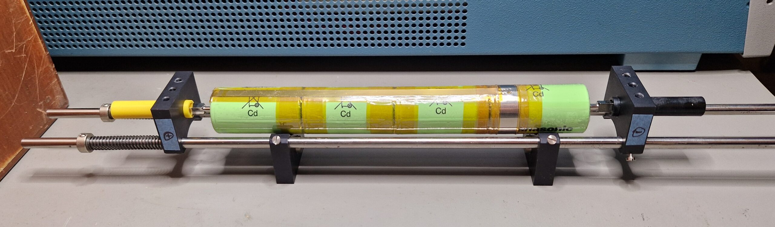
My experimental setup for battery charging and monitoring: Robbe charger, switch-mode power supply, Tektronix TDS 3034B oscilloscope with a P6139A probe and TCP202 current probe. In the center part of the image, the charging fixture for the Ni-Cd battery is shown. Not shown in picture: digital multimeter HP 34401A. Top left: Rubidium Precision Time Base (not used for this experiment, just casually laying around)Quick-and-dirty assembled Ni-Cd battery fixture from optics parts. The electrode contacts are just standard 4 mm banana plugs inserted into 4 mm banana couplings.
My charging/discharging setup looks as follows: the switch-mode power supply (JAMARA Germany DC Regulated Power Supply, Output: 13.8 V & 0-20 A) is connected to the charger. The charger output is then connected to the battery pack fixture. For my battery fixture, I used some spare optics parts I had at hand. The spring-loaded electrode helps to keep the battery in place and also helps to provide a reliable electrical contact. The recharger was powered on and set up to the “DISCHARGE -> CHARGE” mode, which is recommended by the Robbe manual. The battery under test had a remaining voltage of about 2.4 V and was discharged with a current of about 0.1 to 0.3 A. As soon as the battery was discharged to a certain threshold voltage (e. g. 1 V open circuit voltage), the charging cycle began by a slow ramp-up of the voltages and currents. After few minutes, the rapid charging is reached at approx. 6 V and 4.5 A (about 30 W), which corresponds to a charge rate of 1.5 C. I could observe some kind of a charge duty cycle, where the current flow stopped for a certain amount of time before continuing again – perhaps for thermal management purposes. The charging process took about 60 minutes, the estimated restored battery capacity (= transferred charge) was in the order of 3000 mAh. The temperature of the setup was monitored during the charging process with a thermal camera, however the battery pack didn’t heat up significantly in comparison to the mentioned THS 720 internal battery charger. The voltages were monitored by a digital multimeter HP 34401A and an oscilloscope Tektronix TDS 3064B, the current was monitored by a Tektronix TCP 202 current probe. This allowed me to estimate the power demand during the charging process.
Measured voltage of the empty Ni-Cd battery pack
Ongoing discharge, monitored via an oscilloscope
Charging ramp-up shortly after charging begins
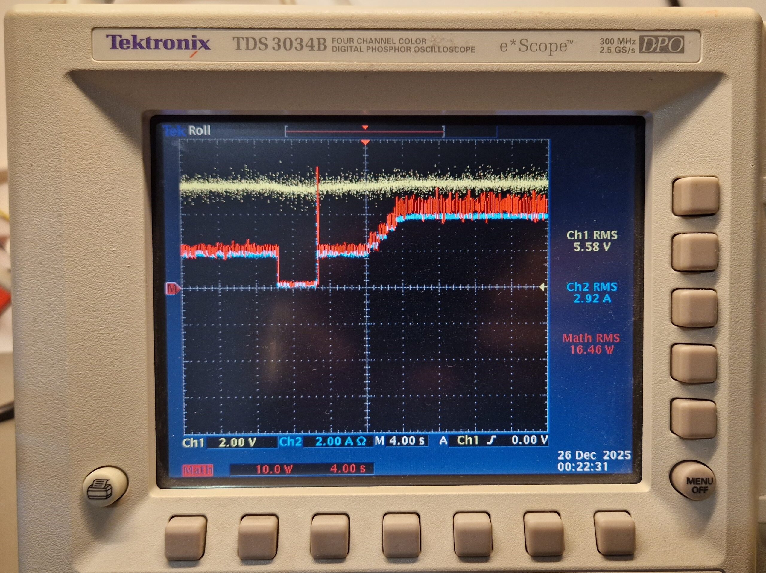
Charging voltage, current and power at maximum output (6 V, 4.5 A)
Charging has finished
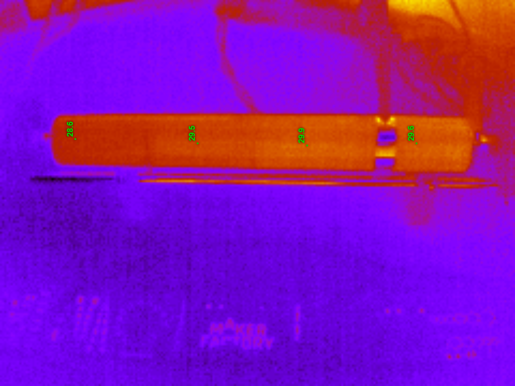
Thermal image (IR) of the experimental setup
Temperature measurement during Ni-Cd rapid charging
Thermal image of the battery setup, taken few minutes later
I was surprised how well and how fast this recharging process went. The DIY battery pack proved to be suitable alternative to the original battery pack Tektronix THS7BAT. Unfortunately, the Ni-Cd batteries age and need to be replaced over time. However, an inexpensive alternative with modern-day parts for a reasonable amount of money (~30 … 40 EUR) can be used to replace the original battery pack and extend the lifetime of the oscilloscope usage, at least until the internal electronic parts start to fail (e. g. the opto-couplers of this scope).
Tektronix THS 720, operational with a fresh recharged battery
My vacation has come to the end and I arrived safe and sound back home in Braunschweig, Germany. Everything went well and it’s time to reflect the past four weeks and draw an outline for the bike tour in summer 2026.
My Bike Tour 2025 from Malmö (Sweden) to Bergen (Norway) – a total distance of 2120 km in 22 days! Source: Google Maps
This was one of the best tours and vacations I ever had. I’ve cycled the Scandinavian leg of the North Sea Cycle Route No. 1 – around 2120 km (= 1317 miles) in 22 days from Malmö (Sweden) via Helsingborg, Halmstad, Göteborg, Vänersborg, Mellerud, Bengtsfors, Töcksfors, Ørje (Norway), Halden, Fredrikstad, Oslo, Drammen, Tønsberg, Langesund, Kragerø, Arendal, Grimstad, Lillesand, Kristiansand, Mandal (at midnight), Lyngdal, Farsund, Liknes, Flekkefjord, Egersund, Ogna, Stavanger, Haugesund, Leirvik, Bergen and many more in-between cities. The weather was perfect for cycling – mostly sunshine or friendly with occasional rain, I liked and enjoyed the lakes, the sea and the landscapes. I’ve met wonderful, kind and like-minded people along my route.
I’ve tried to document my voyage in daily blog posts. There was an overload of so many impressions almost every day! So I tried to keep up with the happenings on road. Thanks to the very good cell phone connections along the route, I was able to do it in a minimalistic fashion on my smartphone. I’ve made over 3000 pictures and it was difficult to make a good selection, because almost every picture has its own story… I hope that some future-travellers will find those information useful to plan their own route. If you have some specific questions about this bike tour, please write me an email at DH 7 DN [at] darc [dot] de. I’m checking it on a weekly basis due to low traffic – but I’ll answer asap!
Training my legs
The preparations for this particular tour started in winter 2024/2025. I’ve been doing cardiovascular training during the winter/spring months and basically cycling on average 5-6 days per week. I was able to reduce my weight from approx. 100 kg to about 92…94 kg in order to get in shape. The training was nothing special, just the “usual” 60 minutes or 25 km of fast cycling per day. I’ve tried to keep it up with the training plans just two days before the journey started.
Planning the tour
I started planning this bike tour on paper in February/March 2025. The main inspiration came from the German website Radreise-Wiki / Nordseeküstenradweg Norwegen and the OpenCycleMap.org website. It was a very good guide what to expect, huge thanks to the creators and writers of the wiki and the map. However, there is no “recipe” for such a week-long journey – one has to pick out suitable tracks. It’s impossible to see everything in a limited amount of time. So I’ve done some research on the internet (Google for bike tours to Norway), watched some YouTube videos (can highly recommend Bicycle Touring Pro YouTube Channel), checked the Wikivoyage for possible tourist spots and few others. A fellow cyclist showed me a nice travel guide booklet for this route, which I didn’t have on my mind. Anyways – much time went into preparation and creation of a plan or “time schedule” in order have a “tailored” bike tour. You can try to do it “by the numbers” but be aware of some possible real-life obstacles.
However, the route planning on a computer looked very easy but was hard to execute on-site. I’ve miscalculated the distances with errors of as high as +30%. For example: a 100 km daily cycling distance estimated by the map tool proved to be 120-130 km at the end of the day. I didn’t have experience with hills and what average speeds to expect. Now I’ve got some data for future tours… terrain with hills: 10-11 km/h on average, flat terrain: 14-16 km/h on average. It is easy to be wise after the event!
The previous bike tours to Denmark helped me a lot to estimate the travel effort. Having some knowledge Denmark’s roads, terrain, people, accommodation and railways made it much easier for me to travel. The first two days at Malmö/Copenhagen proved to be necessary, because starting such a tour on arrival would have been rather difficult: preparations and packing all the stuff took me about three full days and the immediate journey from Braunschweig to Travemünde via regional trains was very stressful. One has to calm down a bit in order to get in the mood and start a bit relaxed.
Starting the tour
The first three to four days on route are usually used for adaption to the new country and terrain. Trying not to overstretch, getting a healthy routine and finding out the right speed are the primary goals. If anything hurts – no problem, as long as you don’t ignore it and try to overcome it with painkillers. I had some problems with my toes on the feet during the first couple of days. I took care of it and it was gone. Getting a healthy amount of sleep (6-7 hours) every night was very important for the cycling performance. I was able to cycle 100 km per day on a constant basis, sometimes 120-130 km per day were possible without having pain in my legs. That kind of performance was necessary, otherwise the planned schedule would have been in vain.
Riding a bike with too much weight
One major problem I had on route was a too heavy bike. The bike itself has some 18 kg. The fully packed pannier bags add some 25 kg, water and food may add another 10 kg of additional weight. So the total weight of me including the fully packed bike was up to approx. 140 to 150 kg! I always travel too heavy but this proved to be extremely difficult in the hills of Norway. I had to push my bike uphill a lot and tried to shed some weight by carrying a bit less food and water. I was considering of sending stuff back to Germany by mail but luckily it wasn’t necessary. I’ve carried a lot of unnecessary or unused stuff, such as backup clothing (“just in case” but the “case” came maybe with 5% chance), portable fan (for hot nights inside of the tent), a camping chair (used it only 3 times, great for full trains with no free seats), a basket (to keep the pannier bag in shape, worst decision ever), two steel bottles (for extra water, were sometimes useful but took too much space in the bags) and some other gadgets/tools (bags, tent pegs, USB cables, rags, …). The weather proved to be very favorable at 15 °C during nights and 20…25 °C during days. I’ve used my sleeping bag on three occasions in some shelters but most of the time I have used the Merino Wool Sleeping Bag Inliner as a “sleeping bag” inside of my tent. If it gets a bit colder at night, one can put on some additional clothes to stay warm, otherwise no “classic” sleeping bag is necessary. This can save up a lot of precious weight and volume and make life a bit easier.
For the future travels to Norway, I would have to lose some weight (down to 80…85 kg) and shed some equipment to get down to ~130 kg of total weight. This would improve my cycling experience a lot.
Bike performance, maintenance and technical difficulties
About 6 weeks prior to the tour, I’ve let my bike workshop inspect my tour bike, the vsf Fahrradmanufaktur TX-1200. They have replaced the front wheel, the pedals (both had worn-out bearings) and brake pads. Besides that, everything else looked fine. On route, I’ve had two flat tires on the back wheel due to riding a very heavy-loaded bike on coarse gravel roads. The little tiny and sharp stones sliced the tire over time and pointy shards were able to puncture the hose. I’ve replaced the tire and hose and had no more problems for the final ~300 km of the route. Another difficulty arised with the Pinion P.18 gear under heavy loads in combination with steep roads. Pinion is just great – I like it very much. It has some awesome properties I don’t want to miss anymore. However, when riding a 140 kg bike uphill in 10-15% slope in the 1st or 2nd gear, I’ve noticed some randomly occurring slippage, which is generally a bad sign. In order not to damage the Pinion gears, I’ve been cautious and pushed the bike uphill instead, some 20-50 meters before resuming the pedaling. There were no issues on flat terrain or hills up to 7% slope – lucky me. I’ll ask my workshop to look into this during the next inspection. Just be aware of the huge torques on steep roads – such conditions can easily damage any type of gear system (e. g. Roloff or Derailleur).
I’ve performed some minor maintenance on my bike during the tour. My Brooks saddle was greased every week due to heavy moisture (sweat, salt, rain). It’s necessary to keep the saddle dry and clean, otherwise it will start losing its shape or build up some cracks in the leather. The Brooks saddle was very comfortable and I could sit on it 8 hours per day without having soreness (however, try to change the sitting position every 20-30 minutes to relieve the buttocks, otherwise you will get a sore ass). It was necessary to replace brake pads once due to excessive breakings in the hills. The salty sea water spray caused some visible corrosion which needs to be taken care of. Besides that, I’ve greased the Gates belt every 200-300 km with the recommended spray. Some screws got a bit loose so I tightened them occasionally. Other than that, no further bike service or maintenance was necessary.
Camping, daily expenses and Allemannsrett
As I traveled with bike and tent, I spent most nights on camping sites or another places such as benches, shelters, forest and a parking lot. I took a two day stay in a hostel in Copenhagen but besides that, it was mostly camping. The camping prices in Sweden were moderate (20-30 EUR per person and night) and got really expensive in Norway (30 EUR per night, Oslo: 50 EUR per night). In Germany, a camping overnight usually costs between 15-25 EUR per person and night. So avoiding camping sites in Norway was necessary to stay in budget. Why? Because everything else is expensive, too! The food prices are also roughly 30% higher than here in Germany so it’s virtually impossible to keep the budget low if you plan to eat at restaurants. I’d estimate 30-40 EUR per person per day as realistic, however, the costs can double easily with “luxury food” and “premium services”. Other expenses such as transportation costs (by bus, ferries, trains, …), luxury money (eating at restaurant, having an ice cream) or emergency (repairs, replacement of equipment) should be considered in the price range of 300-500 EUR. I’ve spent around 400 EUR per week (= 60 EUR per day) on average and had around 600 EUR of travel expenses (trains, ships) in total. I could have saved some 20% by not buying stuff at gas stations or buying luxury food such as expensive chocolate bars… anyways, I think it’s fine.
The Allemannsrett I’ve expected was a bit different from what I’ve found on route. I’ve found many privately owned properties or signs with “Camping forbidden” where you aren’t allowed to camp over night. Those were exceptionally present along the touristic spots and along the Route 1. About 10 km outside of a town, and perhaps some few kilometers off-route, one could find very nice and appealing camping spot – perhaps at a lake. However, this heavily depended on the region and terrain. I couldn’t take my bike on steep hills or find a camping spot in a bush. The mosquito plague wasn’t as bad as expected. I was visited by them but sleeping in a tent helped a lot. I had some luck with pecks (killed them before they could bite me) and inspected my body two times per day for any intruders or parasites. The insects aren’t our enemies (except mosquitoes), they are just looking for a food source and being lured by our presence (e. g. breath, scent, noises). The bushcrafters on YouTube can give you some tips how to behave correctly in the forests and how to deal with the insects. Just be aware of this – better be safe than sorry.
Roads and traffic
95% of the cycling roads in Denmark, Sweden and Norway were in an exceptionally good condition. I’ve never had such a good riding experience. The car drivers were very kind and cautious. They were overtaking cautious with about 1.5 meters of distance to me. I was warned by horn on three occasions: once by an Italian camping van driver, once by some crazy/drunk gang having a good time and once when I entered a tunnel where cyclists and pedestrians were not allowed. I felt safely on the roads and was very confident that I would finish the tour alive
On the other hand, there were some minor issues on route: missing signs put me on wrong route multiple times per day. Some construction sites (e. g. near Oslo) made a detour necessary. The ferries were great except that one in Øysang. I’ve noticed that many Swedish and Norwegian pedestrians walk on the “wrong side” of the road. This confused me a bit because I wasn’t used to drive on a collision course with a pedestrian. One just needs to signalize an overtake with the left arm and everything will be fine. Absolutely no need to bell and yell at them!
What’s next?
My wallet needs to heal. Usually I spend 600-800 EUR for such a three-week bike tour but this tour was expensive for sure. I’ll try to find a good compromise between travel expenses, accommodation and “premium stuff” next year. My next year’s journey would continue from Bergen to the north towards Lofoten. Lofoten aren’t a “cycling paradise” due to its mountain-like terrain and harsh weather conditions, however, I’d like to travel to the northern parts of Norway and perhaps reach Nordkapp by 2027. That would be awesome! The return route would be either by ship (Hurtigruten) or by train/by bus. I’d use more ferries to deal with crossing the fjords and try not to cycle on roads or through tunnels “by any means necessary”. Unfortunately, my vacation time is limited every year to 4 weeks during the summer time so I’d expect some 1500 km in 3 weeks at best with one additional week for arrival and departure. Right now, I’m just enjoying the good time I had in Denmark, Sweden and Norway and looking forward to return next year…
I have been very busy during the past 3 months. I’ve prepared some blog posts but had no time or motivation to finish and publish them. Usually my blog posts have several hundreds or thousands of words with images which can be very time consuming when compared to microblogging services such as Twitter/X or Instagram and Mastodon. I’ll try to keep it brief this time 🙂
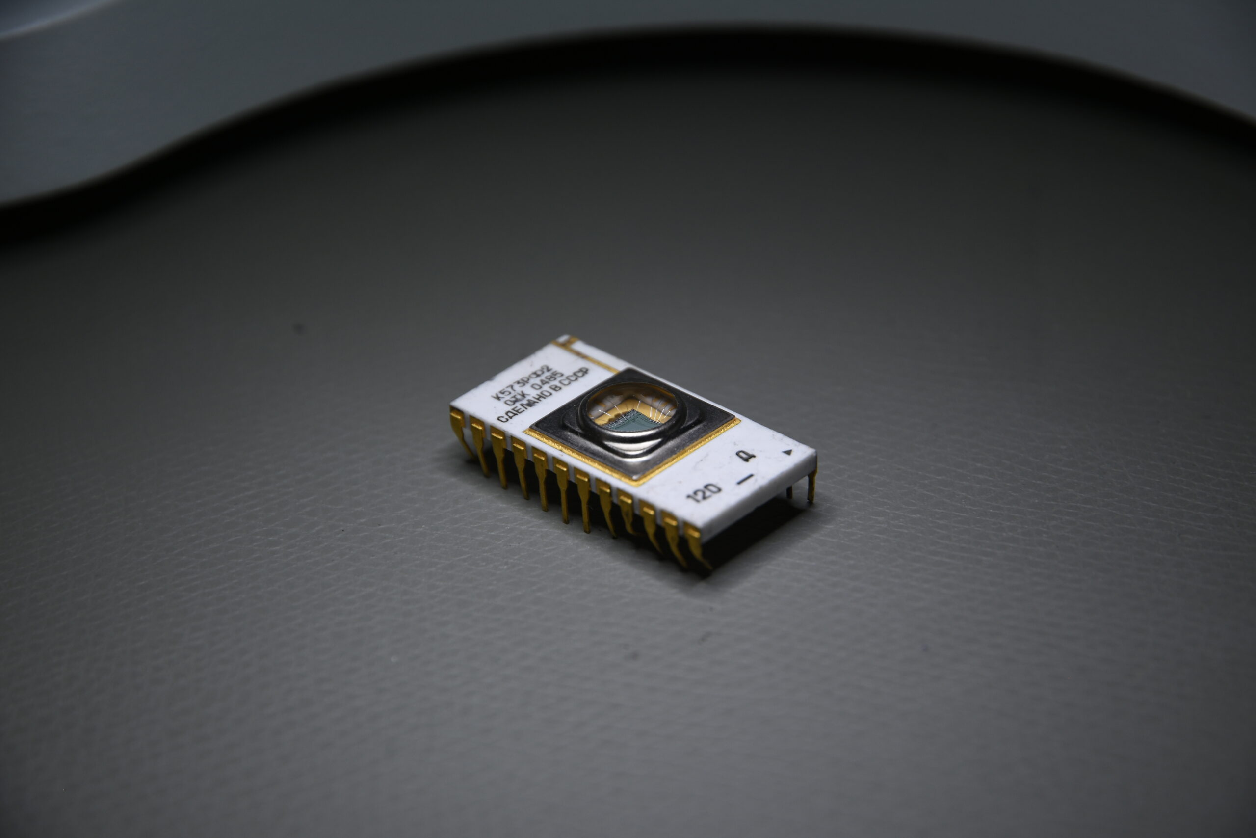
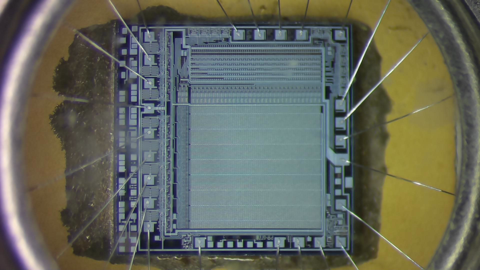
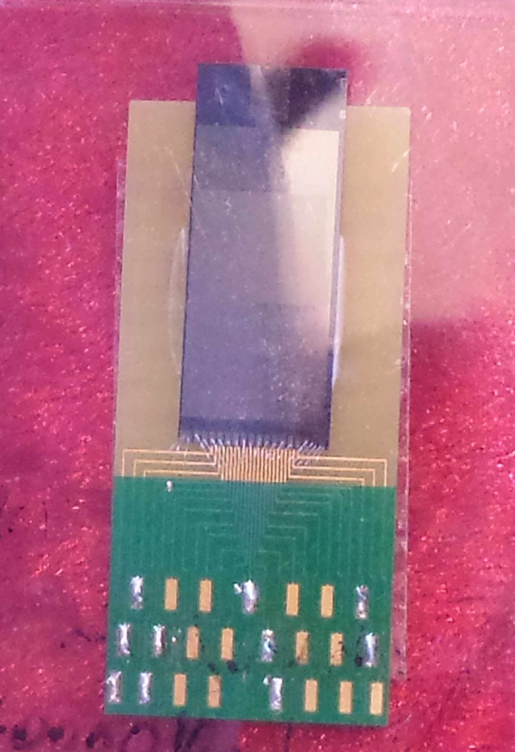
The recent dumpster diving dropped off few pieces of Soviet technology: a type K573RF2 EPROM. In original Cyrillic script it’s written as Κ573ΡΦ2 confused as K573PO2 or K573P02.
K573RF2 Soviet EPROM – Perspective View
K573RF2 Soviet EPROM
K573RF2 Soviet EPROM
Erasable Programmable Read-Only Memory (EPROM) retain data even after the power has been switched off. There is an interesting Wikipedia article on EPROMs which I’d like to refer to. EPROMs were used during the microcomputer era of 1970s and 1980s as non-volatile memory and have been replaced by modern memory types such as EEPROMs and Flash Memory. This particular integrated circuit (IC) from Soviet era is probably a clone of a 2716-type of EPROM which has been manufactured by Intel during the 1970s. The date code of this particular unit suggest a manufacturing date either in week or month 04 of the year 1985.
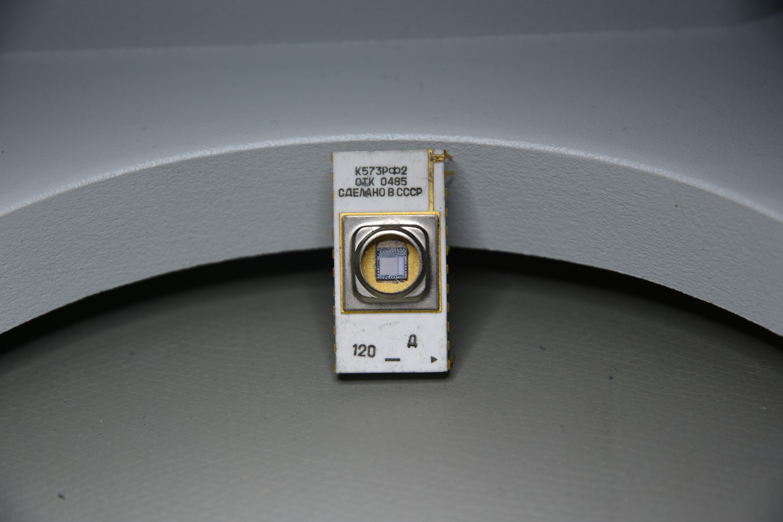
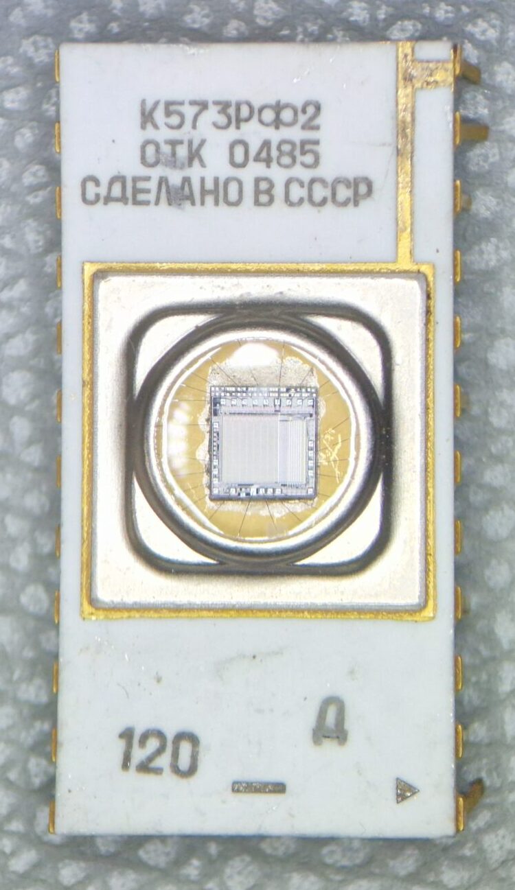
K573RF2 view on the integrated circuit
K573RF2 Soviet EPROM – IC view
I tried to get a good shot of the integrated circuit which can be seen through the quartz window. Unfortunately, I don’t have a suitable microscope with the necessary magnification optics to resolve more details. EPROMs have a distinct fused quartz window which permits to shine ultraviolet light (UV) on the silicon chip. UV light exposure erases the programmed memory cells which can be re-programmed again. Well, can’t say much about it. You can see the bonding wires and the arrangement of the memory cells. One could trace the bonding wires to the pin out and reverse engineer it. The packaging is probably made of alumina and with gold plated pins – this may indicate a military version of this IC?
I’ve found a datasheet for K573RF2 (K573P2-2716) and tried to translate it K573P2-2716_en via Google Translate. Have fun!
New addition to the lab! I bought Giovanni’s book via Amazon because it’s really epic. You can find freely downloadable, high-quality ebooks on his website: http://www.k100.biz/e-Books.html
Tektronix Epic Oscilloscopes by Giovanni Becattini. An epic book!
Unfortunately, it’s a “niche-topic book” but every vintage Tektronix aficionado will appreciate it. As an owner of 400, 500, 2400, 7000 and 11000 Series Tektronix Oscilloscopes, this book is just a must-have. Well-spent 70 EUR!
Thank you Gianni, your books are truly well-written, informative, beautiful and inspiring.
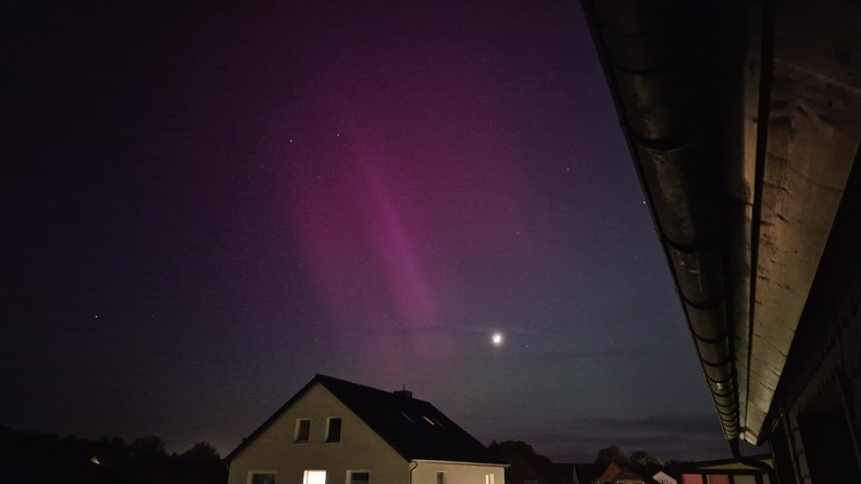
Earth got hit by a Coronal Mass Ejection from our Sun’s activity region AR3664 yesterday. Polar lights were spectacularly visible in most parts of Germany. My friend Michael woke me up around 23:30 CEST (= 21:30 UT) and I immediately rushed to the outside. After taking few (bad) pictures with my smartphone, I moved back to my apartment and observed the natural spectacle from my balcony. We even saw the International Space Station passing over us – a very eventful evening.
Visible Aurorae in Braunschweig, photographed with Samsung Galaxy S22 (2024-05-10): Image taken from the nearby street heading to the north. Unfortunately the street lights show some lens reflections
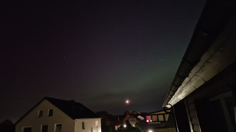
The geomagnetic storm isn’t over yet, we might be able to observe further polar lights tonight! I’ll try to catch some photographs with my DSLR camera!
Visible Aurorae in Braunschweig, photographed with Samsung Galaxy S22 (2024-05-10): Image taken from my balcony heading to the westVisible Aurorae in Braunschweig, photographed with Samsung Galaxy S22 (2024-05-10): Picture taken heading to the west
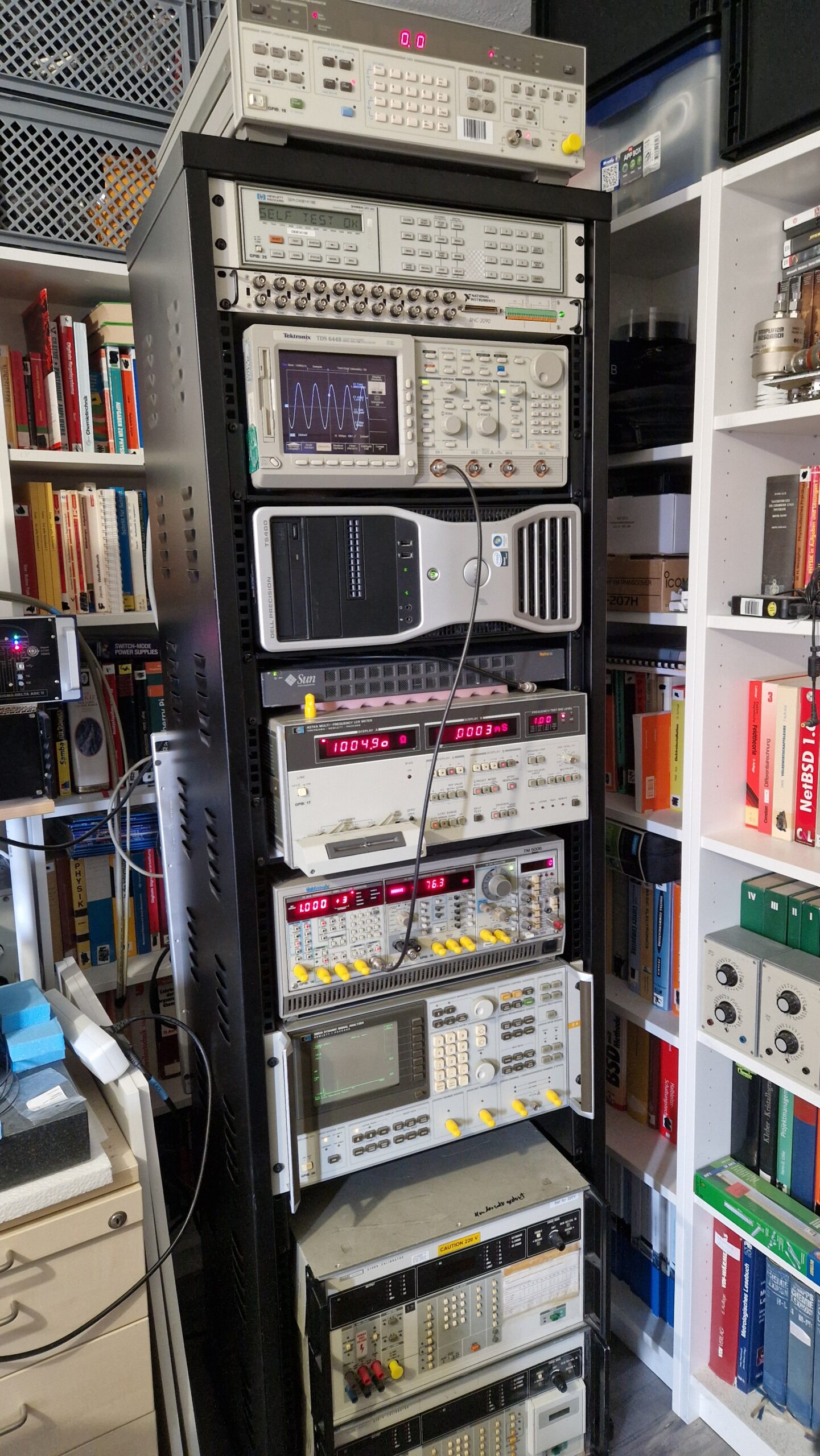
Yes, I have some kind of a Gear Acquisition Syndrome. Yes, I’m a Test Equipment Anonymous. Yes, I love Test Equipment! 🙂 However, this was bothering me for quite some time. The 19″ equipment was laying all over the place and I had some difficulties using it, since the instruments were bulky, scattered and there was no logical order as soon as I wanted to perform measurements. Luckily, a colleague of mine gave me a hint to buy a very cheap 19″ (42 HU) rack mount. This would solve few problems and also introduce new ones (more space for more equipment! Just kidding…). Anyways, I bought the rack mount and after few weeks of procrastinating, I finally equipped it with my 19″ sized test equipment. I’m pretty happy how it turned out. The most heavy parts are located at the bottom and lighter equipment is located at mid to top. It’s stable enough and won’t tip over and it can be easily moved around.
19″ Test Equipment rack mount.
Almost all instruments can be controlled remotely either via GPIB or RS232. An older Dell Workstation will be controlled via Windows Remote Desktop. Instruments from top to bottom are listed as follows:
HP 3325B – A 20 MHz frequency generator with some interesting features for audio testing
HP 3488A – Switch unit equipped with different modules. It’s used for automated, accurate and reliable signal switching or signal routing – it really depends on the used relay cards. I got few of them over the past years, e. g. types 44470A (10 CH multiplexer), 44471A (10 CH general-purpose relay module), 44472A (dual 4CH VHF switch module), 44473A (4×4 Matrix switch) and 44474A (16 bit digital I/O)
NI BNC-2090 is coupled with NI PCI-6110 (PCI multi-function-I/O-card with 4 analog inputs (12 bit, 5 MS/s per channel), 2x analog out, 8 digital I/O)
Tektronix TDS 644B, 4 CH, 500 MHz, 2 GS/s digital real-time oscilloscope. It’s a bit overkill for my audio-type applications – an excellent instrument for displaying waveforms, even RF stuff. A very useful feature is a GPIB interface for remote control and screenshot hardcopy (no need to use the disk drive)
Dell Precision T5400 workstation PC. It’s a 2007 era workstation which I bought probably around 2010 as a second hand PC. I used it like… forever. It was replaced by a faster workstation back in 2020. I haven’t dumped it because of the DVD burner and slots for 3x PCI and 3x PCIe cards. This makes it very valuable when it comes down to using data acquisition PCI cards from early to mid 2000’s era with a Win 7 or Win 10 operating system. Unfortunately this unit consumes a lot of power – it tends to heat up and it’s having thermal management difficulties during hot summers. Few of the ECC SD-RAMs failed over the past years but luckily they have been replaced easily. I tried to equip the three PCI slots with my oscilloscope cards, however, there were some serious thermal issues. I didn’t want to fry the cards so I put them inside of an external PCI expander system
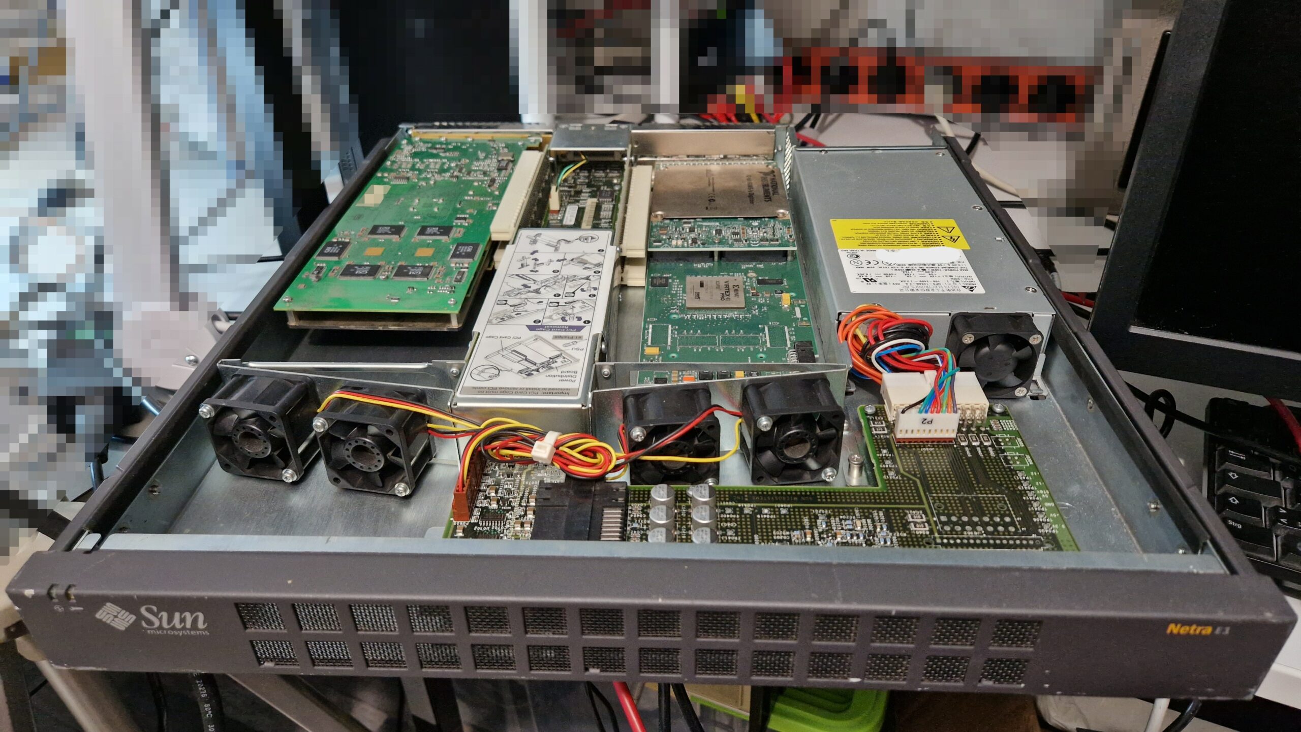
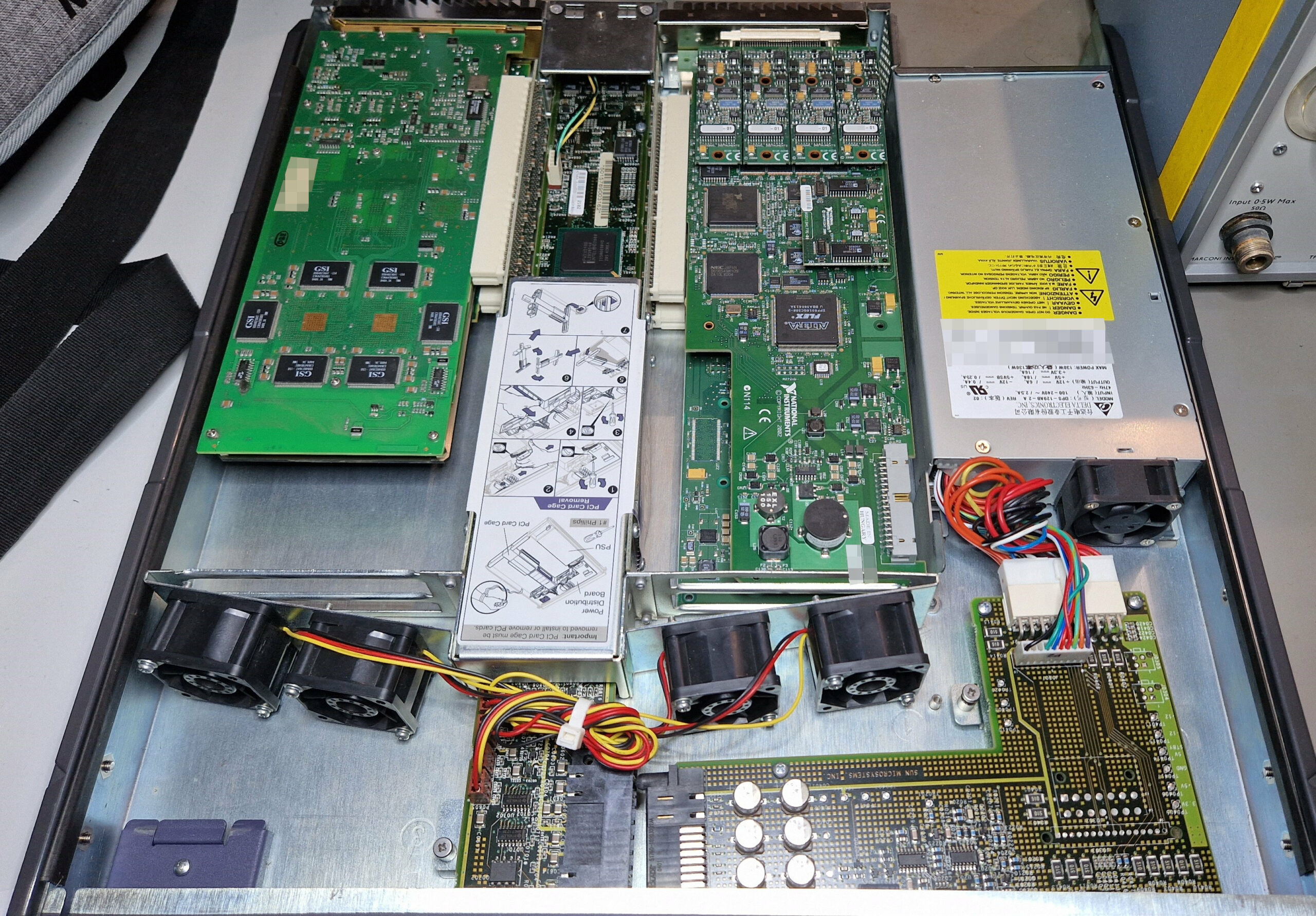
Sun Microsystems Netra E1. After having thermal issues and space problems inside of the Dell T5400, I was looking for a better solution to put the cards in a separate chassis and operate them via a PCIe/PCI bridge. Few solutions exist today, however only few are viable due to hardware/driver compatibility or power delivery constrains. The cheap expansion cards (mostly from China) can’t always deliver the 25-75 W of power to the oscilloscope card. In my case, as soon as the oscilloscope card demanded more power, the PC system crashed. After browsing eBay and looking for National Instruments’ “PXI-like” external chassis solution, I found Sun Microsystems’ Netra E1 as a viable option – however, the price was hefty. In retrospective, I’m glad I bought it because it was ready for use and it saved me a lot of time and trouble. The installation was super easy as PCI/PCIe bridge drivers exist at least since Windows XP. A downside of Netra E1 are the really loud fans. They work relentlessly at full speed; however, they keep the power-hungry cards at acceptable temperatures around 50-60 °C in comparison to 75-80 °C inside of Dell T5400!
Sun Microsystems Netra E1 – PCI Expansion System
Sun Microsystems Netra E1 – Top view.
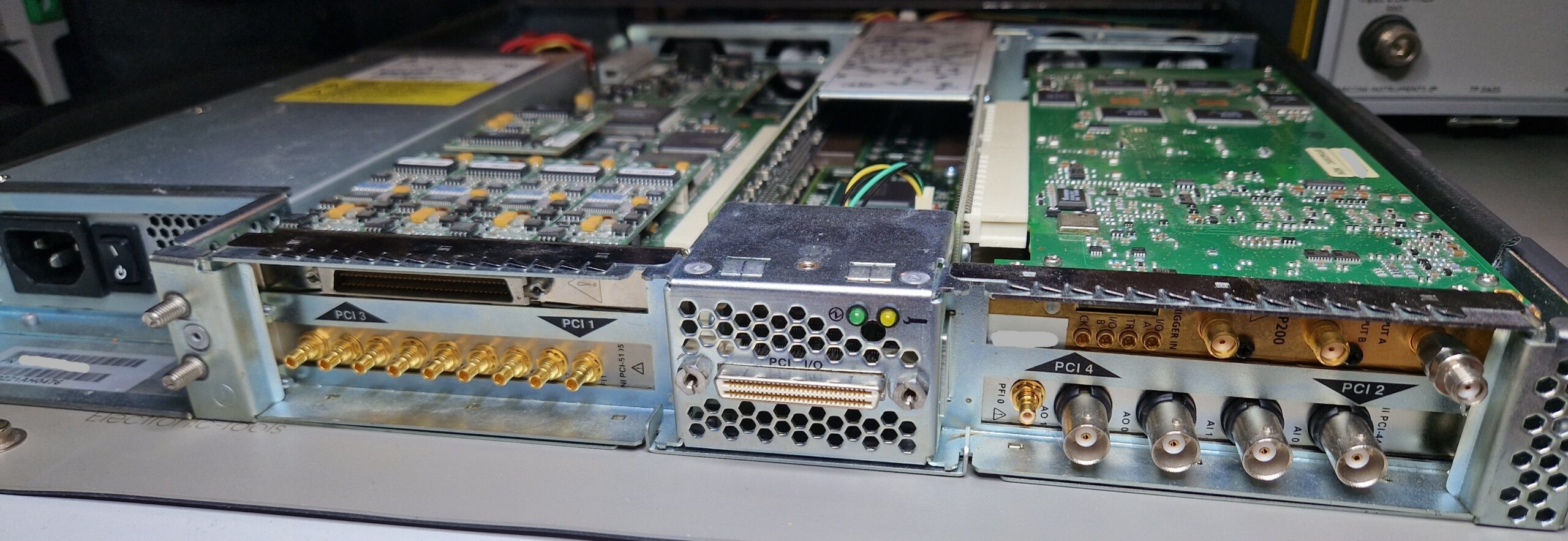
Sun Microsystems Netra E1 – Back view.
Unfortunately, Netra E1 is obsolete technology and no replacement parts exist on the 2nd hand market. Those units were produced around the year 2001 as an expansion system for Sun’s Netra Servers. I might be wrong about this but IIRC their PCI expansion product line was acquired by a company called MAGMA somewhere around mid 2000’s. MAGMA was specialized in building PCI Expander Systems for the Pro Tools Digital Audio Workstations (Pro Tools by Avid Technology, famous tor their audio/video editing software). eBay has some offers with MAGMA expansion chassis up to 16 PCI card slots, however they come at an unrealistic price of $500 to $1000, at least for a hobbyist budget. Anyways, beside the three existing PCI slots inside of the Dell workstation, I was able to put all of my four “power hungry” PCI cards (full length) inside of the 19″ chassis
NI PCI-6110: multi-function I/O card
NI PCI-5105: 8 channel, 12-bit, 60 MS/s digitizer/oscilloscope with up to 60 MHz analog bandwidth
NI PCI-4461: dynamic signal analyzer, basically a $10k sound card, still produced today – according to NI, it can be bought until 2024-12-31!
Agilent/Acqiris AP200: 1 channel, 500 MHz, 2 GS/s high-speed digitizer/averager card (used in radar tech or mass spectrometers)
Yokogawa/HP 4274A Multi-Frequency LCR Meter. I have a bunch of HP fixtures for components, unfortunately the LCR meter needs a repair. Should be hopefully an easy fix since the errors appear after warm-up. Fun fact: The Japanese government was very restrictive and protected their markets in the early days. In order to enter the Japanese market, companies from foreign countries such as United States were obliged to “team up” with a local Japanese manufacturer so they could sell their products in Japan. I guess HP teamed up with Yokogawa and Tektronix had a partnership with SONY. That’s the reason why there is occasionally a double company logo on some pieces of test equipment.
Tektronix TM5006 chassis equipped with
Tektronix FG5010, 20 MHz frequency generator (GPIB-controllable)
Tektronix AA 5001, audio analyzer capable of measuring Total Harmonic Distortion (THD), also GPIB-controllable
Tektronix SG505, audio frequency generator with exceptional ultra-low distortion sine-waves, perfect for audio amplifier testing
Tektronix DC 503, digital counter (doesn’t work, needs a repair)
HP 3562A Dynamic Signal Analyzer. A very capable FFT analyzer e. g. for audio and vibration testing and frequency response analysis in the µHz … 100 kHz regime
Fluke 5100B/5101B Calibrators. They can provide AC and DC voltages and currents and also resistances for calibration of up to 5.5 digit DMMs. Unfortunately, both need repair (power supply issues). Currently they are not in use – I’m hoping to repair them either later this year or maybe in early 2025
Surrounded by the rack mount are my book shelves with many books about physics, chemistry, operating systems and other stuff. A HPM 7177 digitizer can be seen at mid-left. There are only three cables left which are connected externally to the chassis: 230 V power, GPIB and Ethernet. I could replace GPIB with an NI GPIB-USB and Ethernet with WiFi. This would of course simplify the cable management but I’m very happy how everything turned out. I’ll need to find some lifting feet for the rack mount since it’s a bit overloaded with ~200 kg of equipment and it could cause damage the floor and the wheels over time.
Most of the test equipment seen here has been acquired during the past 3-4 years. Some pieces were really cheap (< 100 EUR), others rather expensive (> 300 EUR). It will be used for my laser interferometer and accelerometer calibration project which I plan to build in the future.
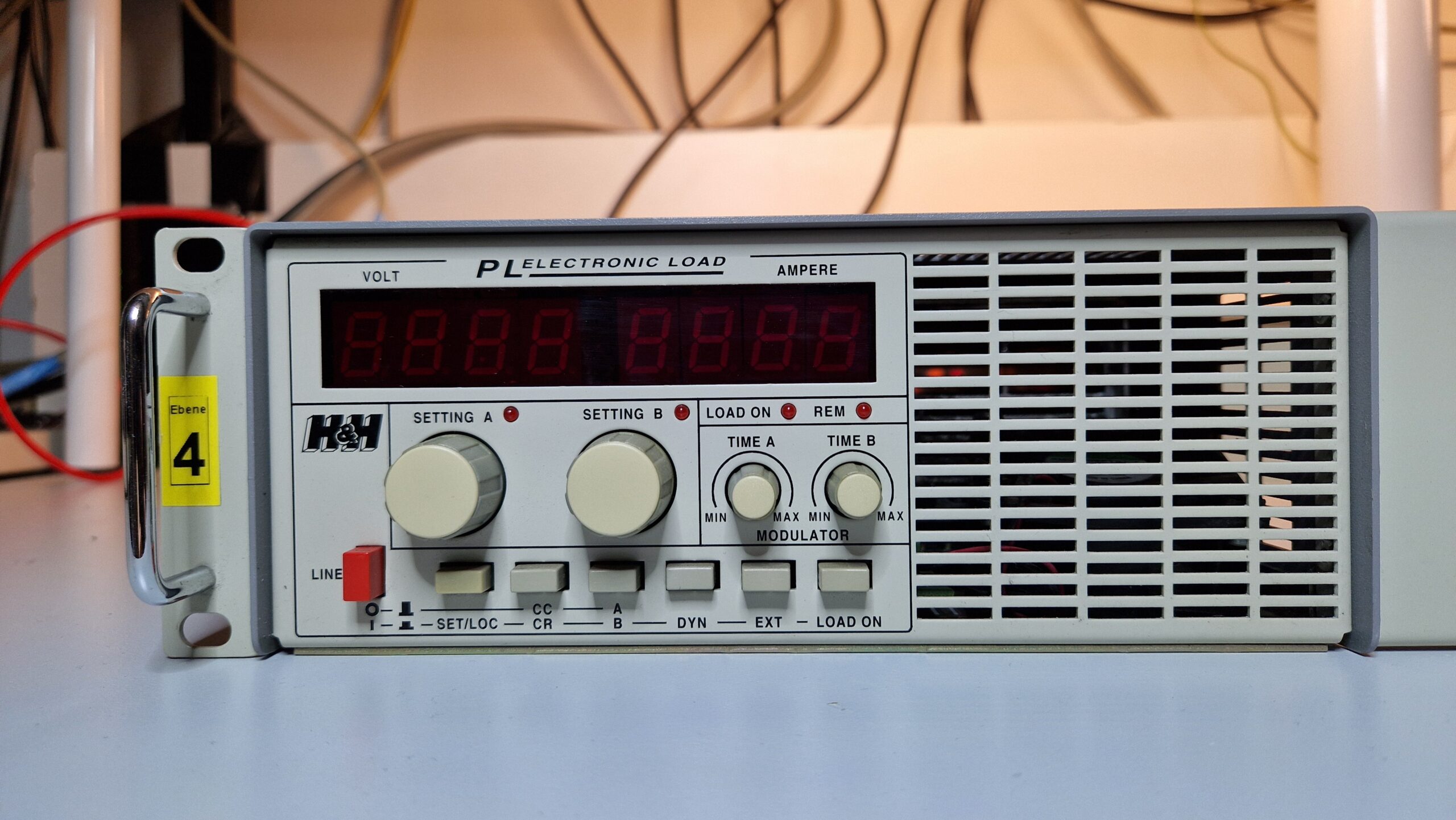
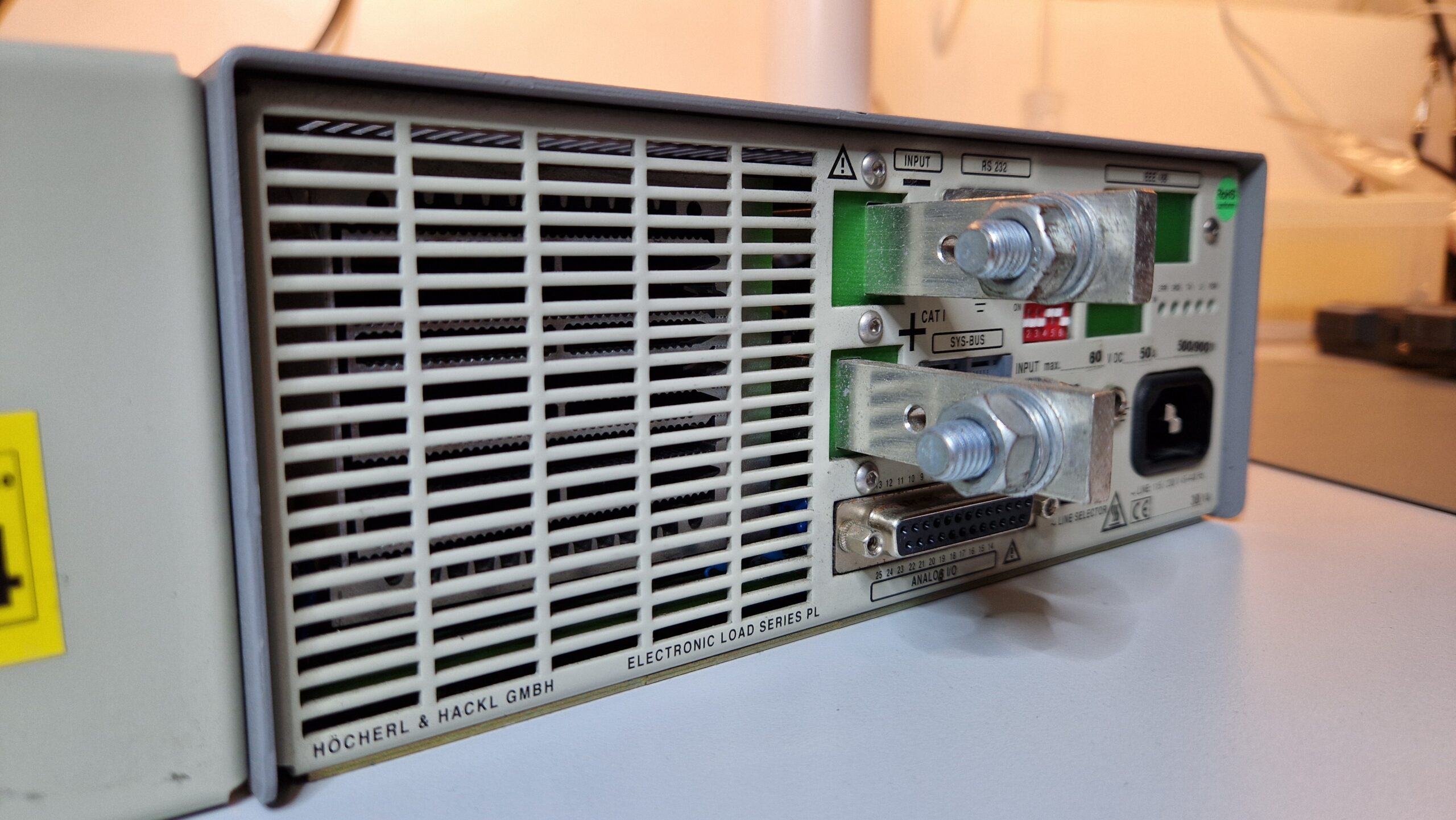
I bought a Höcherl & Hackl PL506 DC electronic load just recently. It’s a nice piece of equipment to test switch-mode power supplies (SMPS) or any DC power sources like solar modules or batteries. I will need few of those for Tektronix SMPS repairs. As far as I can tell, DC electronic loads are rather rare and expensive units. So I grabbed one on an auction site for a very decent price compared to current offers (which is crazy, they ask 600…1000 EUR for such unit).
Höcherl & Hackl PL506 front panel.
Höcherl & Hackl PL506 back side.
After unboxing and shaking the unit, I noticed a strange noise. Since it’s easter holidays here in Germany, I thought it was some kind of a “Kinder Surprise Egg” time!
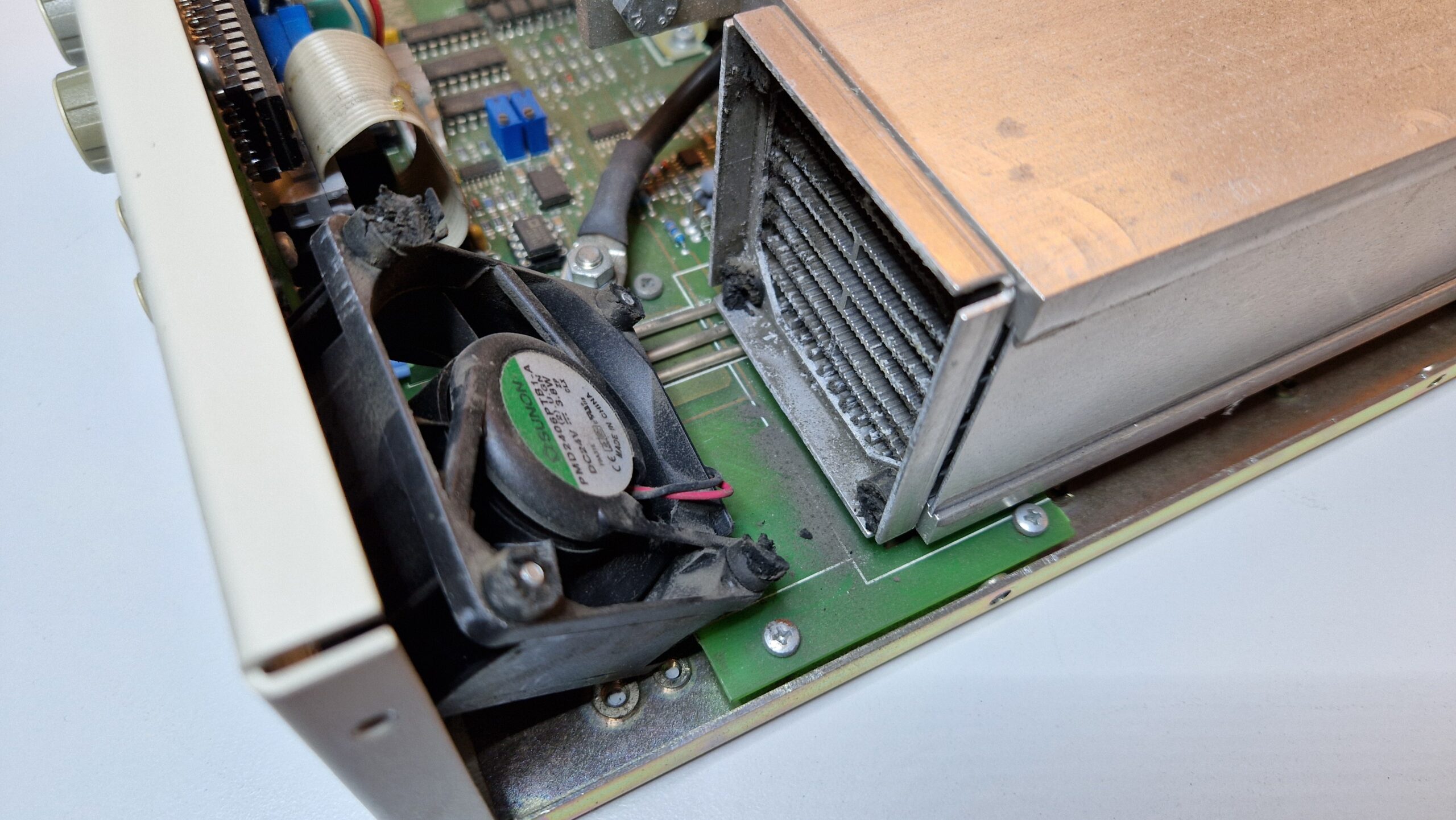
But no, I was disappointed. No easter eggs 🙁 It was the fan which broke off. I looked for other damaged parts and defects but there were none. No signs of burned parts, bad electrolytic capacitors etc. Looking good inside!
Höcherl & Hackl PL506.
H&H PL506 – The unit was shipped like this. The rubber vibration isolators broke and the fan fell off.
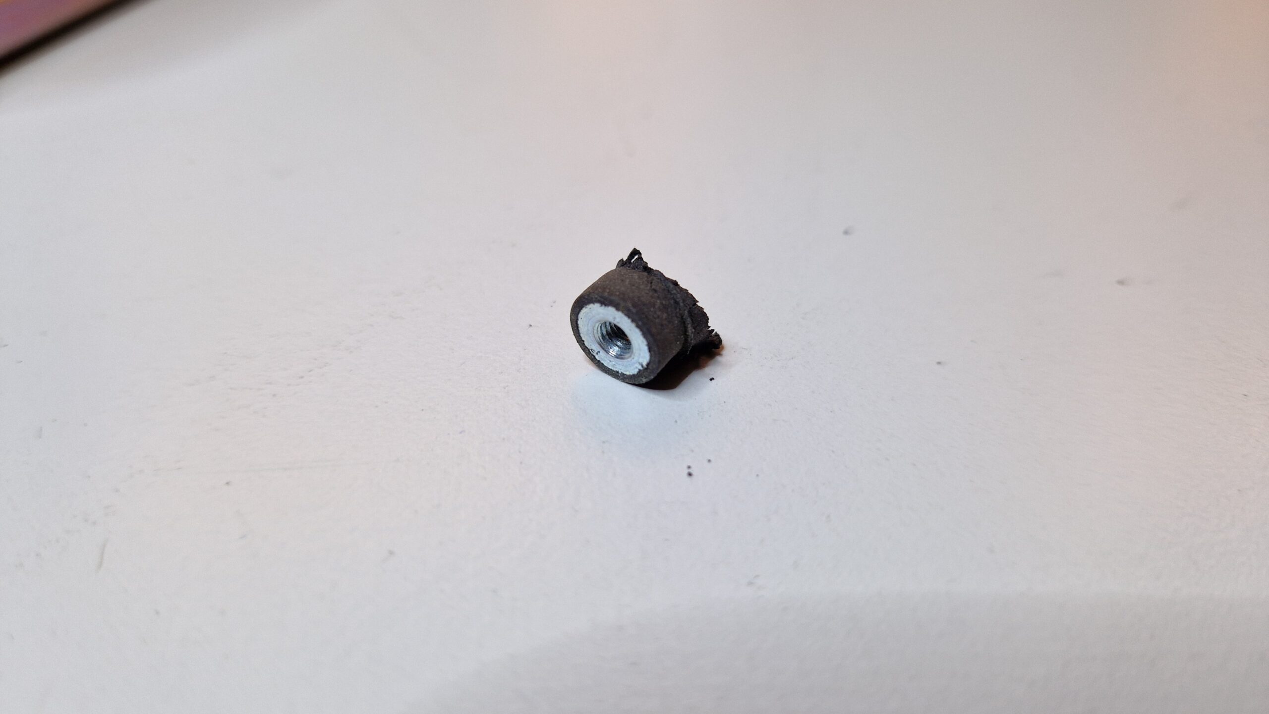
The vibration isolators probably became brittle over the years and broke during the transport. The fan fell off and had to be reattached. The front panel buttons are a bit crusty, too and will need to see a maintenance one day. The heat sink could need a clean-up, too. Build-up of dust and dirt diminishes heat transfer and can cause either performance issues or overheating of power dissipating MOSFETs.
Rubber dampener with metal thread insert.
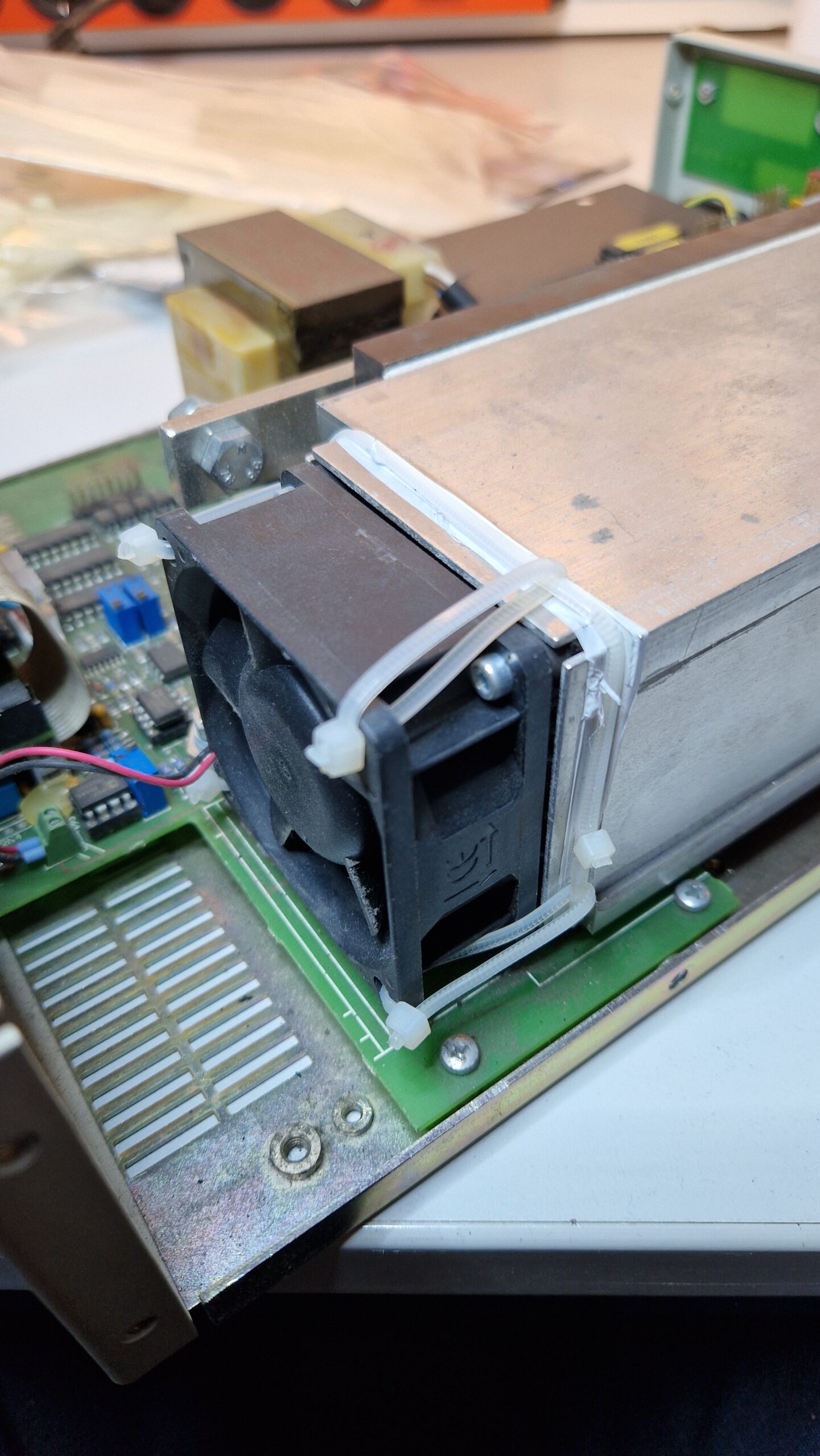
I was looking for a suitable replacement in my electronics parts bins but found nothing. I used zip ties to reattach the fan to the heat sink. The unit was fixed in less than 10 minutes.
Problem was fixed with zip ties.
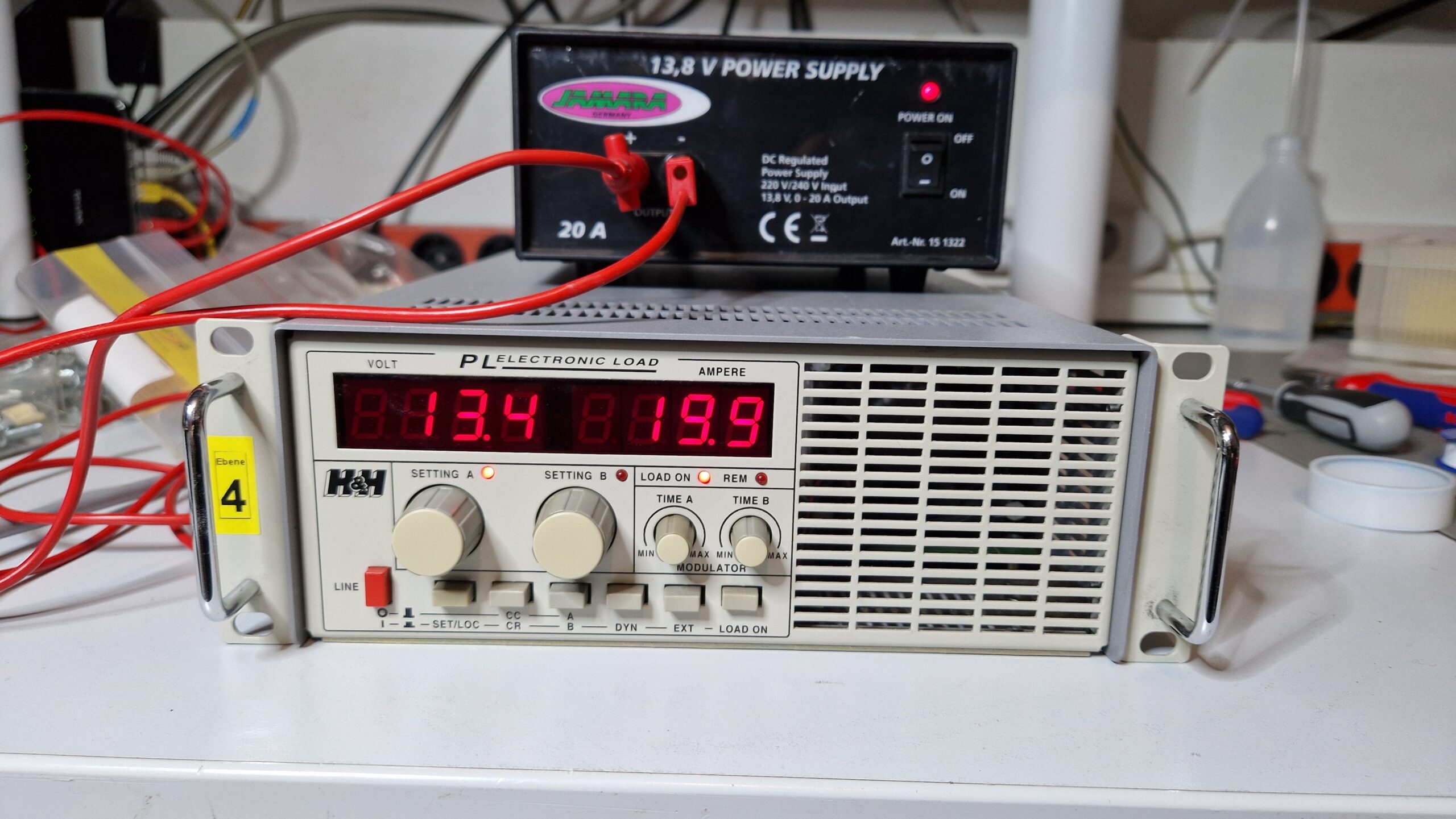
A quick test with a random 13.8 V SMPS was successful. I was able to load 19.9 A at ~13.4 V which corresponds to ~267 W output power of the SMPS. This DC electronic load is capable of dissipating 500 W continuously or up to 900 W short-time. This was a short-time test with 4 mm banana cables since I didn’t have proper high-current cables at hand.
Höcherl & Hackl PL506. Testing a 13.9 V / 20 A power supply.
Very nice addition to the lab. Hope this will be useful for future repair and maintenance projects!
Tektronix TDS 3034B four channel color digital phosphor oscilloscope.
A “new” oscilloscope arrived in the lab just recently thanks to my friend Matt, who relayed the offer to me. It’s a wonderful instrument from the early 2000’s era: a Tektronix TDS 3034B Four Channel Color Digital Phosphor Oscilloscope. The oscilloscope’s analog bandwidth is specified at 300 MHz with a sample rate of 2.5 GS/s per each channel. It has a ton of options (e. g. FFT, 3LIM, 3TRG) and a communication module with VGA monitor output and GPIB/Ethernet/RS-232 for communication and control. There is also a battery compartment, however, the battery was not included. The “Waveform Intensity” knob simulates the intensity control of an analog oscilloscope with a cathode ray tube – therefore a “Digital Phosphor Oscilloscope” or DPO. The size of the oscilloscope is very convenient and perfect for a desk use – doesn’t take much space and it’s fast and responsive compared to my older Tektronix TDS 754D oscilloscope.
Tektronix TDS 3034B back side with battery/probe compartment.
I was able to set up the communication to my PC via GPIB (IEEE 488). Since I already had the Tektronix WaveStar Software for Oscilloscopes installed on my Windows 10 PC, I was able to quickly transfer screenshots/hardcopies, measurement data and sample data from the instrument to my PC. No diskettes or USB drives were needed. It is possible to control the oscilloscope remotely which is absolutely fantastic for measurement documentation and measurement automation purposes! It’s a great addition to the lab and it will serve to me as my daily workhorse among other oscilloscopes, of course.
Tektronix WaveStar for Oscilloscopes. Easy way to transfer screenshots and data from Tek TDS 3034B to a Windows PC.
Bandwidth Upgrade
It seems to be very common (even nowadays in 2024) that the oscilloscope manufacturers design a generic oscilloscope parts which can be used for different models. The oscilloscopes are then assembled with similar to identical hardware components (presumably because it’s cheaper manufacturing-wise) but the measurement capabilities are determined either by hardware (jumper settings) or by software (locked/unlocked options). For example, Rigol DHO 800/900 Series Oscilloscopes can be upgraded from 70 MHz to 100+ MHz via software. Thanks to Matt, he gave me a hint that the guys at EEVblog have figured out how to perform an upgrade of the Tektronix TDS Series oscilloscopes to different models. So already having an excellent 300 MHz & 2.5 GS/s oscilloscope at my fingertips, I was curious if I could upgrade it to the 3064B model which has 600 MHz analog bandwidth and 5 GS/s sample rate. I tried out the EEVblog’s upgrade procedure and it seemed to work without bricking the oscilloscope. I’ll just quickly summarize the procedure here.
*IDN? query via GPIB.
Tektronix TDS 3034B boot screen.
Boot up the device and set up the communication via GPIB (e. g. GPIB address and talker/listener mode). Connect the device to your GPIB controller
I used the National Instruments GPIB-USB-HS controller device along with current NI’s GPIB drivers (driver version doesn’t matter much, you could also use the VISA drivers from Keysight, Tektronix or Keithley). The TDS 3034B Firmware Version was v3.39
The communication between the PC and the oscilloscope was established with NI Measurement & Automation eXplorer’s (NI MAX) own GPIB Instrument Communication. I guess you could use any GPIB communication software, e. g. pyvisa for Python
Check whether the oscilloscope responds to the *IDN? query. If yes, proceed, if not – try to find the problem and fix it (obviously)
Send the following commands to the oscilloscope PASSWORD PITBULL MCONFIG TDS3064B
Just send (write) the commands in the order as shown above! Do not use a “GPIB query” since there will be no response action from the oscilloscope. Upper/lower case letters don’t matter.
Now power-cycle the oscilloscope (turn it off, wait few seconds and turn it on again). It should boot up with a new screen and new model. If it doesn’t show the new model, something went wrong with command transmission via GPIB. As far as I could tell, some models accept only different MCONFIG-commands, such as “MCONFIG TDS3054” without the letter “B” at the end. Anyways, after sending the commands via GPIB and power-cycling the oscilloscope, it should show up with the new model
Changing the TDS model will result in an uncompensated waveform. I observed a DC offset and noise on my CH1 through CH4 waveforms post-update. The solution to this problem is quite easy: wait some time (at least 10-15 minutes) for a warm-up and perform the Signal Path Compensation (SPC), which can be found in the Utility → System Config → Cal
menu. This will perform an internal calibration where the noise and offset errors are compensated. The oscilloscope should be ready for performing measurements afterwards
*IDN? query after BW upgrade.
Boot screen after BW upgrade.
Waveform pulse post-upgrade. Sample rate is at 5 GS/s.
Tek’s Signal Path Compensation.
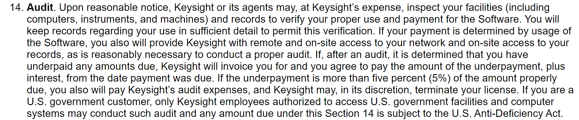
That’s how it worked out for me. It took me just few minutes to convert a Tektronix TDS 3034B into a TDS 3064B. I’d recommend to check out the linked EEVblog thread for further information on the TDS 1000/2000/3000 Series upgrades. Of course I can’t be held responsible if you try it out and damage your instrument (e. g. calibration data or warranty is lost or the device is bricked) since I’m sharing this information and tried it out on my own oscilloscope. This is solely done at one’s own risk! Please be careful when trying out this procedure and please read the EEVblog thread prior to changing the instrument. Always make backups of your oscilloscope firmware prior to changes. Also hacking the device in order to use unlicensed software options is… well… “illegal”… I guess… Keysight’s Agents will hunt your PC down! 😉
Excerpt taken from the Keysight N1500A EULA. This is not a joke (well, it’s a well-known meme), see it for yourself: https://helpfiles.keysight.com/csg/N1500A/License_Agreement.htm
Checking the Oscilloscope Analog Channel Bandwidth
I did some initial bandwidth testing with my Leo Bodnar Fast Risetime Pulse Generator. The pulser generates repetitive 10 MHz square waves (~1 Vpp) with a rise time of around (30 ± 2) ps. It can be used to easily test the oscilloscope’s analog channel input bandwidth. The analog bandwidth of an oscilloscope can be calculated as follows:
So a measured 10%-90% rise time of \(t_r = 1.000 ~\mathrm{ns}\) results in an analog bandwidth of \(0.35/(1.000 \cdot 10^{-9} ~\mathrm{s}) \approx 0.350 \cdot 10^9 ~\mathrm{Hz}\) or 0.35 GHz which is basically 350 MHz. So prior to the bandwidth upgrade we were expecting an oscilloscope bandwidth of ~300 MHz at a 2.5 GS/s sample rate, post-upgrade it should be around ~600 MHz and a 5 GS/s sample rate. I’ve measured the rise time of all four channels in order to see if there are any significant differences between them. The oscilloscope settings were as follows: Coupling: DC, Termination: 50 Ω, Trigger: External, Acquisition Mode: 64× average per acquisition at 10k points and 5.00 GS/s. The trigger was delayed by approx. -10 ns.
Tektronix TDS 3034B CH1 risetime.
Tektronix TDS 3064B CH1 risetime.
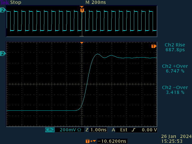
Tektronix TDS 3034B CH2 risetime.
Tektronix TDS 3064B CH2 risetime.
Tektronix TDS 3034B CH3 risetime.
Tektronix TDS 3064B CH3 risetime.
Tektronix TDS 3034B CH4 risetime.
Tektronix TDS 3064B CH4 risetime.
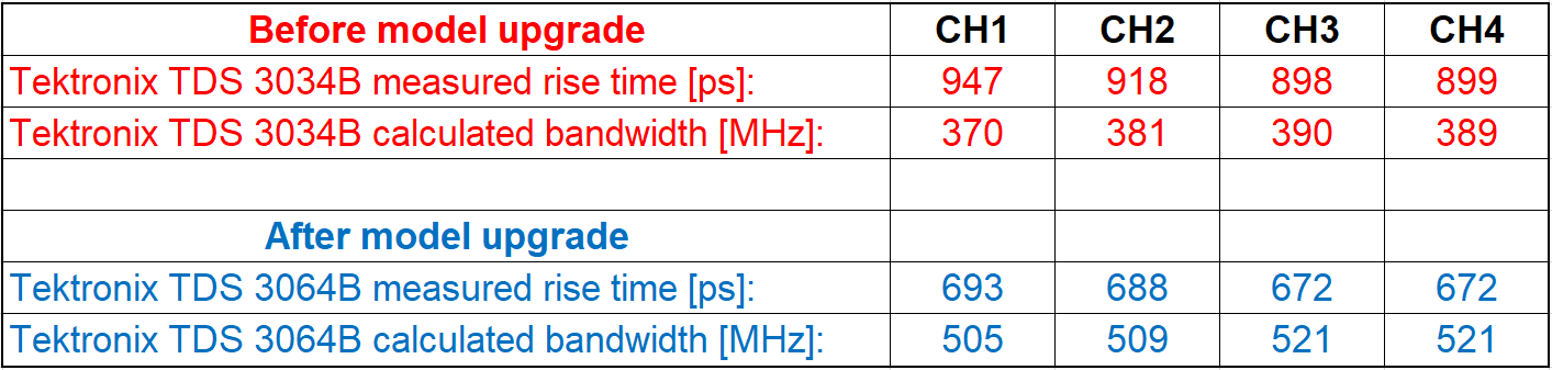
The measurement results are summarized in the table below.
Analog bandwidth calculations from measured rise times for each oscilloscope channel. Comparison between Tektronix TDS 3034B before model upgrade and after model upgrade to TDS 3064B.
As we can see, the full bandwidth of 600 MHz for a Tektronix TDS 3064B has not been achieved. However, there is a measurable improvement. Channels 3 and 4 seem to have a slightly higher bandwidth than channels 1 and 2. The rise time measurements deviate on each acquisition so I would estimate an uncertainty in the rise time measurements of approx. ±10 ps. I also wonder if the overshoot/undershoot calculations are correct. I’ll have to look into this manually, since the data samples can be exported in a CSV file.
Conclusion
Nevertheless, the bandwidth upgrade was successful! 500 MHz analog bandwidth at 5 GS/s is more than enough for my needs before stepping into the GHz time domain regime. And no need for a battery if there is a food compartment in your oscilloscope! Tested successfully with carrots! 😉
It’s currently cold outside (-8 °C) here in Germany and I skipped my cycling tour yesterday. Instead I got myself some stuff to play with during the cold and dark winter days.
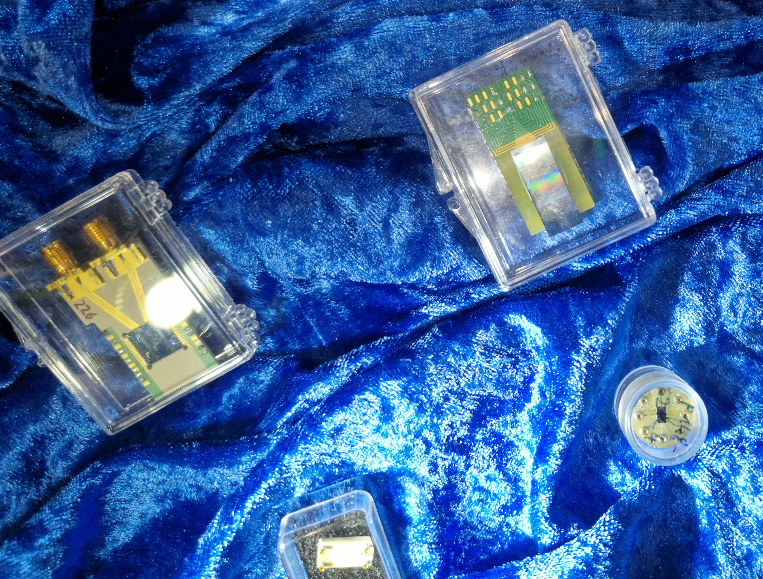
Some new gadgets on the desk.
A “new” handheld oscilloscope Tektronix THS 720 (STD) appeared in my lab! It had a dead Ni-Cd battery so I replaced it with a new one. It seems to work, however, it also seems to have the usual aging issues with optocouplers. Channel 1 shows some DC offset while Channel 2 looks fine DC-wise. The price for this scope was really “OK” (<200 EUR), it’s great for troubleshooting switch-mode power supplies due to fully isolated oscilloscope input channels. It has a built-in multimeter to check voltages simultaneously – great tool for repairing broken test equipment! Well, this instrument also needs a repair, so it’s some kind of repairception? hmm
On the bottom right, we have four Sprague TANTAPAK® wet slug tantalum capacitors, 820 µF, 20-30 V(DC) each. If they haven’t been abused and aren’t leaky, maybe they will be used as decoupling capacitors for a nanovolt noise measurement of a LTZ1000ACH. Need to be tested for their capacitance, ESR values and leakage current. See Jim Williams’ work on Linear Technology Application Note 124. A HP 10514A mixer can be seen on bottom mid. Bought it out of curiosity, will test it. Top left shows a 10 MHz OCXO for a HP 53131A type of frequency counter. On the left hand side, a SUNSHINE IC socket fixture can be seen. A friend told me it was used along with an ancient SUNSHINE EPROM programmer PC card, the one with an 8-bit PC/XT-bus maybe?
Bottom left shows a Raspberry Pi 5 (8 GB) with a cooling fan. Raspi5 was announced in November 2023 but I couldn’t buy it in online shops because there were none available. It took them almost 6-7 weeks to restock their supply. I didn’t want to pay high prices for a Raspi 5 on second hand markets because the offers were 30-50% overpriced in the order of 130 – 150 EUR (which is crazy!). Will be a nice upgrade to my Raspi 3B standing army. I’ve ordered some accessories such as a cooling fan, the 27 Watt USB-C Power Supply, a black case, RTC battery, Micro HDMI adapter cables and a microSD card.
Raspberry Pi 5 8 GB.
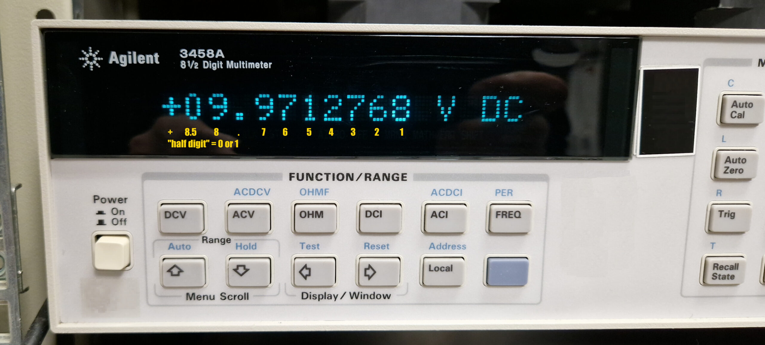
And there is a possible repair project on the horizon. A HP 3458A has presumably lost its calibration data due to a dead battery of the Dallas DS1220Y-150 Nonvolatile-SRAM. The NV-SRAMs in a HP 3458A store settings/preferences and calibration constants. As long as the unit is powered up, the battery coins inside of the Dallas ICs aren’t discharged. However, once the digital multimeter is turned off for a longer periods of time (e. g. months, years), the battery is slowly discharged. Unfortunately, the discharge curve of a NV-SRAM does not show any signs of discharge when measuring its voltage – instead the battery voltage drops suddenly below a power-up threshold and all stored data is lost. The life time of the battery can last between ~8 up to 30 years and it strongly depends on environmental and usage factors. Therefore: please do backup of your IC contents in order to prevent a potential nightmare.
After power up, “RAM TEST 1 HIGH” message appears. With some luck, the batteries of the calibration data NV-SRAMs may be still alive…
HP 3458A is a famous example but there are also oscilloscopes out there (e. g. Tektronix 2465B/2467B, older TDS Series) with a memory-loss time bomb. I’m currently taking care of ordering replacement NV-SRAMs and will try to revive the unit.
HP 3458A Dallas Nonvolatile SRAM. The DS1230Y NV-SRAMs store the preferences and settings while the DS1220Y-150 type holds the calibration data. If the internal battery of this chip dies, the calibration constants will be lost and the instrument will be out of spec. It will need a full recalibration.
HP 3458A A1-9530 board inspection.
I’ll resume my cycling efforts tonight. It’s no pleasure doing this at -8 °C mostly because of cold wind blowing into the face for about an hour or so. Nevertheless, there is no bad weather, only bad clothing!
The new year is already 5 days old. Nevertheless, happy new year to everyone who reads this blog. As always, I’ll try to post on a regular basis about my adventures in the fields of bike touring, amateur radio and test equipment / gear acquisition syndrome. Keep up the good work, may your projects be fulfilled in 2024. Stay healthy and sound and keep up a positive attitude.
73, Denis (DH7DN)
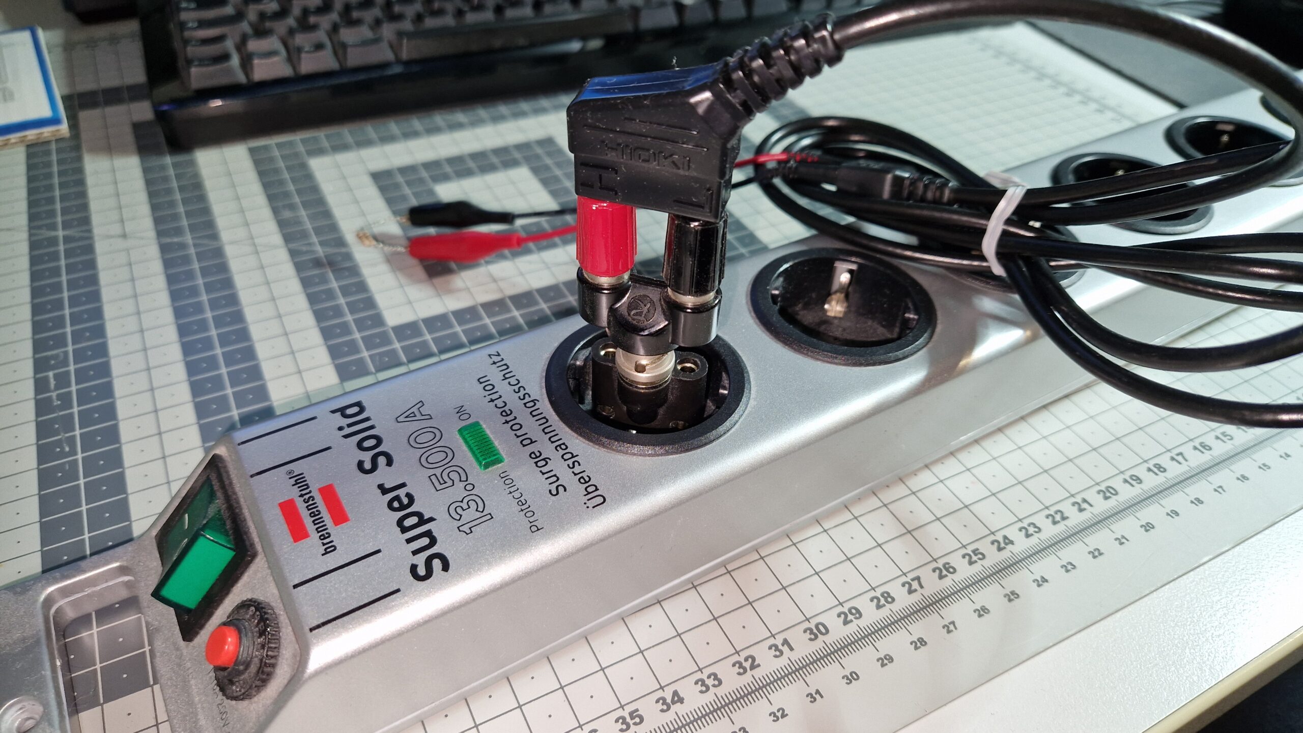
Hiroki test lead with a rather dangerous adaption 😉
I bought a Tektronix 576 Curve Tracer on the second hand market some time ago. Unfortunately, the seller wasn’t able to ship it and he did not live in my region. The pick-up place was near the town of Düsseldorf – a 350 km distance from my place. Oh boy…
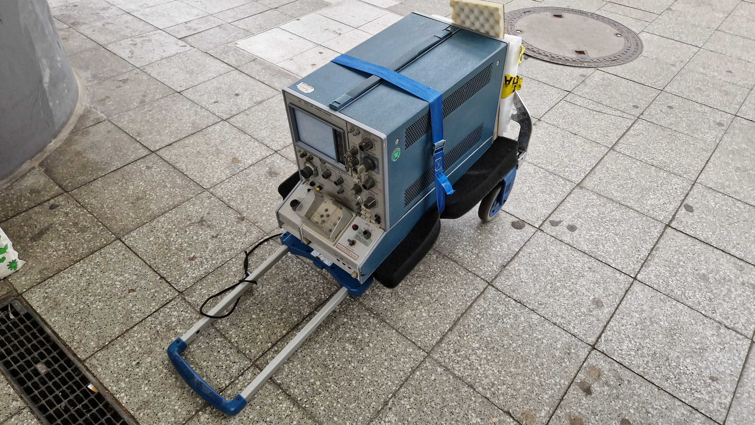
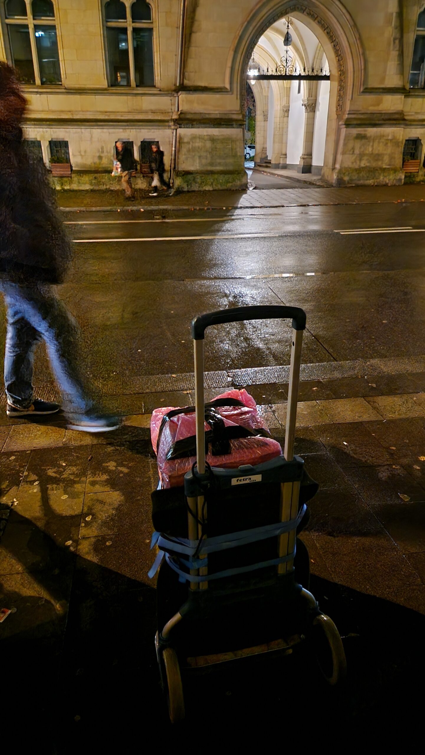
The problem with this particular curve tracer is its size and weight: it can’t be hand-carried for long distances because it’s a 35 kg (~70 lbs) chonker. Even if it’s carried by one person, one has to be very careful not to damage delicate parts and also for health and safety reason when carrying heavy instruments in a wrong posture. Shipping this curve tracer via regular parcel service is almost impossible or very expensive. Since I don’t have a car right now and car rentals are also very expensive, I tried to pick it up and bring it back home by train. The idea was to use a small hand truck for transportation in busses and trains. This way, it should be possible to treat it as luggage.
Well, it kinda worked out somehow! I started my journey in Braunschweig at around 8 am and headed towards the central train station by public transport. Luckily the connecting trains were on time so I reached Düsseldorf at 12 pm. The seller was very kind and agreed to meet at the nearest train station where he handed over the curve tracer with a manual. It took me about 20-30 minutes for packaging and securing the curve tracer with straps.
The Tektronix 576 Curve Tracer was handed over to me on a parking place near Düsseldorf.
Quick and dirty transport in order to escape the rain and get to a dry spot.
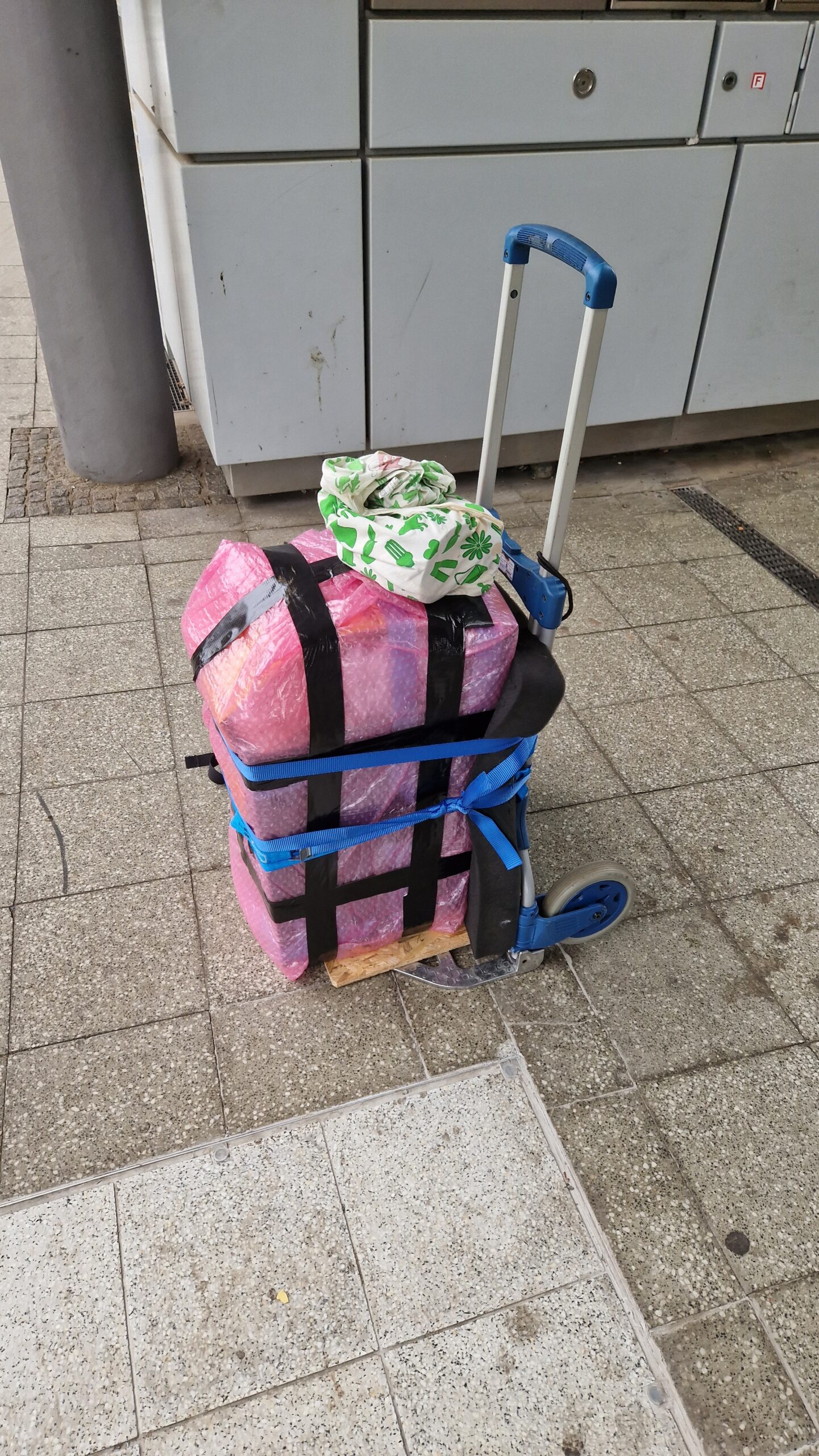
Tektronix 576 properly packed on a train station.
The journey back from Düsseldorf to Braunschweig was much more difficult and was delayed multiple times. However, time was not an issue and I managed to get back home with a 2 hours delay at 7 pm. The total price for travelling by train in both directions was around 70 EUR which is comparable to current gasoline prices for a ~700 km route.
The curve tracer fits very well inside of the luggage compartment.
Some trains were full and crowded.
We had bad weather on this day. However, the Tek 576 was well protected from rain.
I used some cardboard pieces and soft foam to protect the knobs and sensitive parts. Hard foam was used to protect the back side and a grey soft foam mattress was added for additional cushioning. The bubble wrap was used as thermal isolation and rain protection (temperature shocks aren’t good for electronic and plastic parts). The straps were used to secure the instrument so it doesn’t fall over. The blue masking tape is really useful for attaching the cardboard to the housing. The masking tape is very easy to remove without leaving tape residue or peeling off the paint.
Unpacking of the Tektronix 576 Curve Tracer back at home.
Tektronix 576 Curve Tracer taking place at the Tek Cart.
After getting back home, it took me some time to unpack the Curve Tracer. I’ve waited at least 24 hours to power up the unit since it had to acclimate to the ambient temperature. It’s not a good idea to power up a cold instrument which has been exposed to low temperatures for hours. I was very tired after the travel but everything seemed to work out very well.
I couldn’t find any broken or damaged parts. Taking a look inside of the instrument showed no signs of a transport damage. From my experience, such a delicate instrument needs to be handled properly, you can’t always trust the parcel service. Taking care of the transportation is the only way to ensure the instrument will “survive” the move from A to B. Who else didn’t experience the “Courier Transformation” at least once in their life? By the way, it’s a nice pun to the “Fourier Transformation” 😉
As you can see, heavy instruments can be transported by train, at least here in Germany. However, this transportation method becomes very impractical as soon as the round trip times exceed 12-13 hours. Travelling 12+ hours by train is no fun for sure therefore it’s not always a viable method.
That’s it for today. The next blog entry will show some post-power up experiments and shots of the Tektronix 576 innards.
I don’t consider myself as a voltnut. I don’t design precision circuits and I don’t do crazy and expensive things like selecting, binning or matching of super-expensive components (Zener voltage references, foil resistors or opamps). I don’t spend my evenings on Christmas doing circuit simulations in LTspice. However, I like the idea of DIY-ing of an existing precision circuit design and verifying its performance. Thanks to Illya Tsemenko, Marco Reps and the voltnuts all around the world and their endless efforts in searching for the best design for a DIY voltage reference – it is nowadays possible to build a laboratory-grade, high-performance solid state voltage reference using off-the-shelf components which performs very close to their commercial available counterparts and costs just a fraction of its price (perhaps less than 10%). In this self-shaming blog entry, I want to talk about how I totally didn’t build my own voltage reference yet and how I am trying to measure ADRmu based voltage references by using CERN’s HPM7177 high-precision digitizer I also didn’t build myself. Please note: I’m not a metrologist. The reality is much more complex and the devil is always in the details. I hope that the informations provided here aren’t too far off. If so, please consider consulting ChatGPT for further guidance 😉
Voltage references – A quick summary
Voltage references are electronic devices used as a representation of the physical quantity “direct voltage” (DC volts). In the early days of DC volts metrology, voltage references were based on electro-chemical cells (Clark cell, Weston cell) before they were superseded by Josephson Voltage Standards (JVS) during the early 1970s and 1980s. Weston cells are very delicate devices and contain hazardous/toxic materials (mercury and mercury/cadmium amalgam, cadmium sulfate and mercurous paste) and therefore are not the kind of electronics device one wants to keep at home.
Quantum Metrology Porn: PTB’s Josephson Arbitrary Waveform Synthesizer (JAWS) IC (left), Programmable Josephson Junction Series (top right) and Quantum Hall Device (bottom right) as seen on Maker Faire Hannover in 2022.
JVS is the most accurate device for generation of DC voltages, however it’s very complex and expensive due to its needs for very specialized equipment (microwave feed, cryostat, probe, superconducting integrated circuit chip, readout and control system).
PTB’s Programmable Josephson Junction Series IC as seen on Maker Faire Hannover in 2018.
PTB’s Josephson Arbitrary Waveform Synthesizer (JAWS) IC as seen on Maker Faire Hannover in 2018.
There is currently only one viable and affordable voltage reference option for a precision electronics hobbyist: an ovenized Zener voltage reference. This solid state voltage reference design revolves around a subsurface (“buried”) Zener reference with a heater resistor for temperature stabilization and a temperature sensing transistor, which also compensates the temperature coefficient (TC) of the Zener reference. Ovenized Zeners are widely used as a DC volts reference in laboratories and as an integral part of high-precision test equipment such as digital multimeters (e. g. HP/Agilent/Keysight 3458A, Fluke 8588A), calibrators (Fluke 5700A, Fluke 5730A) and ADCs/DACs. They can also be used as voltage standards for digital multimeter calibration, as part of a Kelvin-Varley voltage divider or act as a so-called transfer standard – a transportable artifact with a well-known and predictable properties (stability, noise, TC) in order to “transfer” the quantity “direct voltage” between two laboratories.
Linear Technology’s LTZ1000ACH Ultra Precision Reference.
Building a world class DC voltage reference is difficult
Building a voltage reference based on Linear Technology’s LTZ1000/LTZ1000ACH or its successor Analog Devices’ ADR1000 takes a bit of effort and… money! Almost every serious design relies on precision electrical components because every component contributes to the performance of the future voltage reference. It starts with the printed circuit board (PCB). The voltnuts have figured out how to arrange the components on a PCB in order to deal with thermal gradients and thermocouple effects, electromagnetic interference (EMI), circuit protection and different sources of noise. There are many PCB designs available online, such as xDevs’ KX/FX, Dr. Frank’s LTZ1000 or Marco Reps’ ADRmu. The Gerber files can be downloaded free of charge and can be used for submission to a PCB manufacturer (e. g. JLC PCB or PCBway). You can also DIY the printed circuit board by etching the traces by yourself. Ordering a PCB would be the easy part because you get a very good quality PCB without having to deal with chemicals and drilling holes. Everything else concerning building the voltage reference can be considered as very difficult or even “hard mode”.
Voltnutting equipment. Top: two LTZ1000ACH, Mid: an early prototype of ADRmu, Bottom: Sticker, 3D-printed caps for the LTZ1000ACH (preventing air streams) and a book from Fluke “Calibration: Philosophy in Practice”, 2nd Edition. Thanks to Reps Precision Group (RPG) for design and dissemination of future ppms.
Ordering precision electronic parts isn’t a straight-forward process. In most cases, one has to check multiple online shops in order to find the suitable components. Some parts are really expensive while others are very difficult to obtain. Last time I checked the LTZ1000ACH prices at Mouser Electronics (September 2023), its was around $93 per piece (excluding VAT). The price used to be around $65 per piece before 2020. Speaking of 2020: who doesn’t remember the electronics components shortage which resulted in LTZ1000 lead times up to 52 weeks (Mouser, DigiKey, Farnell, …)? This was a real thing just about half a year ago. Meanwhile, the stocks have been replenished. However, the prices have risen significantly (+30%) compared to pre COVID-19 times. Buying precision electronic parts off second hand market (eBay, craigslist) can be a winner but I would consider this as a gamble . Depending on your source, there is always a risk of buying counterfeit, defective parts or parts with a poor performance. Precision resistors, which are needed according to the Linear Technology’s reference design, are also very expensive ($25..30 per piece, 4 needed) and difficult to obtain. Another difficult to obtain components are the low thermal EMF binding posts (~ $25 per set). I participated in an EEVblog group buy which took about 2 months from placing the order until receiving the binding posts (Thanks to branadic! This was entirely done voluntary by him and free of extra charges). Just be aware of those time and money sinks.
Low thermal EMF binding posts. Thanks to branadic at EEVblog for taking care of the group order from Asia.
Building an ovenized Zener voltage reference ought to be a long-term project of mine. I don’t want to rush things and plan to accumulate the necessary components over time, perhaps during a timeframe of 2 to 3 years. I already have two LTZ1000ACH waiting in my desk but everything else is missing. I need to order the precision resistors, the PCBs, the enclosures, transformer cores and I have to find some time for assembly.
Precision parts have arrived – what’s next?
Once you have obtained the essential parts, you’re ready to do the assembly. But hold on for a second – you have to know what you’re doing and you have to do it very carefully. For example, if you apply too much heat when soldering your precision resistors or LTZ1000 to the PCB, it can result in a disaster. Overheating a precision resistor can either damage it and render the specifications void or introduce an unwanted hysteresis, which makes it either susceptible to temperature changes or drift over time. Those drifts directly influence the stability of the future voltage reference and greatly reduce its performance. Assembly is crucial and early-made errors are punished much later in the future. And don’t forget the obligatory bottle cap in order to prevent air streams. Be careful when handling precision electronics parts: always wear gloves to prevent contamination with grease/dirt and also take ESD precautions. Try to use quality parts over “Chinesium”.
ADRmu
In order to kick-start the project, I was fortunate to grab one ADR1000-based ADRmu for myself, which Marco built and tempco-tuned by himself. I needed a point where I would be able to get started with DCV metrology and to accumulate few thousand hours of operation time. One of the ADRmu’s design goals was to be compatible with LTZ1000(ACH) and ADR1000. ADRmu has protection circuits, a gain stage to shift the voltage from typically 7.2 V to a value close to 10 V and an eXtReMe isolation transformer for common-mode suppression. It’s possible to fine-tune the gain stage with discrete resistors in order to get the voltage output close to 10 V (if necessary). Very interesting features of Marco’s design is the possibility of use of resistor networks with an option for using discrete precision resistors. Resistor networks consist of thin film resistors manufactured in one process, which are thermally coupled through their substrate and hermetically sealed inside of their package. A resistor network has a very stable resistance ratio (e. g. 13 kΩ/1 Ωk) which is crucial for the LTZ1000(ACH) stability. That’s an advantage compared to discrete resistors (e. g. 13 kΩ and 1 kΩ) which have their own TC and drifting characteristics and therefore contribute to the performance of the LTZ1000(ACH) circuit.
Innards of ADRmu, Marco’s voltage reference design.
Once it’s built – the adventure starts
Once you have built your voltage reference, it’s time for the first measurement. Depending on the voltage reference, this measurement should be done with a high accuracy DMM under stable environmental conditions with proper leads. Typically it can be done with a 6.5 digit DMM (HP 34401A, Keithley 2000) or even better ones, such as 7.5 digit (Keysight 34470A, Keithley 2001) or maybe 8.5 digit class DMM (e. g. Keysight 3458A, Keithley 2002, Datron 1281 etc.). During the first several months or maybe during the first year of operation, the voltage reference will show some kind of measurable drift. The magnitude of this drift will be in the range of few ppm (2…5 ppm/year maybe, just to name some numbers).
Voltnutting equipment shown at Maker Faire Hannover 2022: Keithley 2400 SourceMeter (top), HP 3458A (middle), Fluke 5700A (bottom). HP 3458A is running in 7.5 digit mode (d’oh!).
This is a well-known property of solid state voltage references. Initially they drift few ppm over time but settle after many hundreds or thousands of hours of operation. It’s called “aging” and the reasons for aging processes are hidden behind the “semiconductor physics curtains” (changes in mechanical stresses acting on the semiconductor, outgassing and diffusion processes, electrical changes in the circuit elements). Also power-cycling a voltage reference can lead to so-called hysteresis due to thermal shocks which are experienced during powering on/off the oven (having a ΔT of 40-60 °C in a precision semiconductor circuit isn’t very healthy). So the goal is to keep the voltage reference powered on permanently, at least for months or perhaps years. Voltnuts are serious about this issue and rely on uninterruptible power sources (UPS). Good and stable voltage references change in the order of <0.3 ppm per month – not every voltage reference will reach this kind of performance “out of the box”. It is possible to select best-performing Zeners from a production sample. However, it’s an expensive gamble if you plan to select maybe two or three “good ones” out of 20.
In order to get reliable and somewhat predictable results, every voltage reference needs to be characterized in terms of stability, low-frequency noise and temperature coefficient. A voltage reference with an unpredictable drift is basically worthless because it doesn’t meet the stability criteria and therefore doesn’t qualify as a reference or standard. Currently I’m not able to do the noise and TC characterization yet because of lack of a ultra low-noise amplifier and a climate chamber. That’s another rabbit hole which has to be skipped yet 😉
How do you measure the stability of a world class DC voltage reference?
A high-accuracy DMM such as Keysight 3458A has built in a LTZ1000(ACH) as a voltage reference for its ADC. What happens if we measure another LTZ1000 with this kind of meter? We are basically comparing two similar voltage references to each other. Now let’s suppose the DMM’s internal DC volts reference shifts for 1 ppm. As a consequence, the indicator on the DMM’s display would show a voltage shift of 1 ppm. But in reality, we wouldn’t know if our instrument’s internal DC volts reference or our Device Under Test (DUT) shifted! The only way to know which one changed (DUT or DMM) is by comparison between a larger number of voltage references (e. g. 2, 3 or 4). One possibility would be to use two Keysight 3458A to measure one voltage reference. This way it would be possible to identify whether one of the DMMs or the DUT shifted. Since a 8.5 digit DMM is a very expensive piece of equipment, it’s much cheaper to build few more DC volts references and compare them to each other within a group of references.
So the answer to the question would be: one rather compares the voltage differences between multiple voltage references and observes the long-term stability between them. This is usually done with a calibrated high-accuracy DMM or (if you’re a vintage kind of a guy) so-called Null Detector. This way we are gaining confidence in the stability of the DC voltage reference and simultaneously we’re building a calibration history of each unit.
CERN’s HPM7177
I do own a HP 34401A (6.5 digit DMM) which is good enough for 99% of measurements but not good enough for voltnutting or DC volts metrology stuff. 6.5 digit metrology isn’t something I really look forward to do (like some guys over at EEVblog). In order to monitor the stability of my voltage reference(s), I’ll need a 8.5 digit class meter. Since the market for HP 3458A is currently overheated and buying such an expensive device is associated with potential risks (bad or drifty U180 ADC), there might be a possible alternative within a hobbyist’s budget.
HPM7177 sitting there and gaining ppm dust. It’s a beautiful design and very well crafted by A Random German Guy (ifyouknowwhatimean).
Few years ago, CERN TE-EPC group’s member Nikolai Beev has proposed a design of a metrology-grade ADC called HPM7177 which has been published as an Open Hardware project in the meanwhile. HPM7177 is based on Analog Devices’ AD7177-2 Sigma-Delta ADC, Linear Technology’s (now Analog Devices) LTZ1000ACH ultra precision reference and Vishay’s PRND Thin Film Resistors. It’s a single channel ADC card with a native sampling frequency of 10k SPS with a maximum bandwidth of 5 kHz. An effective resolution of 23 bit for a bandwidth below 10 Hz can be obtained. The measuring range is ±10 V with a 30% over-range. A really nice feature are the thermo-electric coolers for temperature stabilization of the temperature sensitive parts.
Two HPM7177 units have been built by Marco. He documented the assembly in one of his YouTube videos. I “inherited” this HPM7177 from That Random German Guy 😉 some time ago. However, I wasn’t able to use it due to lack of time, projects and most importantly: I wasn’t able to do a proper calibration of this metrology-grade ADC. Meanwhile it’s been powered up since March 2023 and a calibration and characterization has been performed in May 2023.
One small downside of HPM7177 is its inconvenient operation: the incoming data is encoded as a 32-bit integer, which it needs to be read out via USB at a fixed sample rate of 10 kHz and post-processed after data acquisition. Recording all samples generates a huge amount of data in the order of 100-250 kB/s. This is no problem for a modern-day computer and Python, however, long-term measurements may generate lots of gigabytes of data very easily. At a certain point it’s becoming highly impractical to save raw data in a human-readable CSV file so one has to consider using different formats such as NASA’s HDF5.
Soon™
HPM7177 has been powered since early 2023. Let’s hope the internal references did not drift too much. Next calibration in 1-2 years will tell.
Alright, this is already too much text I’ve written as an introduction to my voltnutting ambitions. I’ll write another (shorter) blog post how I did the calibration of HPM7177 and share some measurement results. There will also be some integral nonlinearity (INL) measurement results here which I was able to perform with suitable instruments.
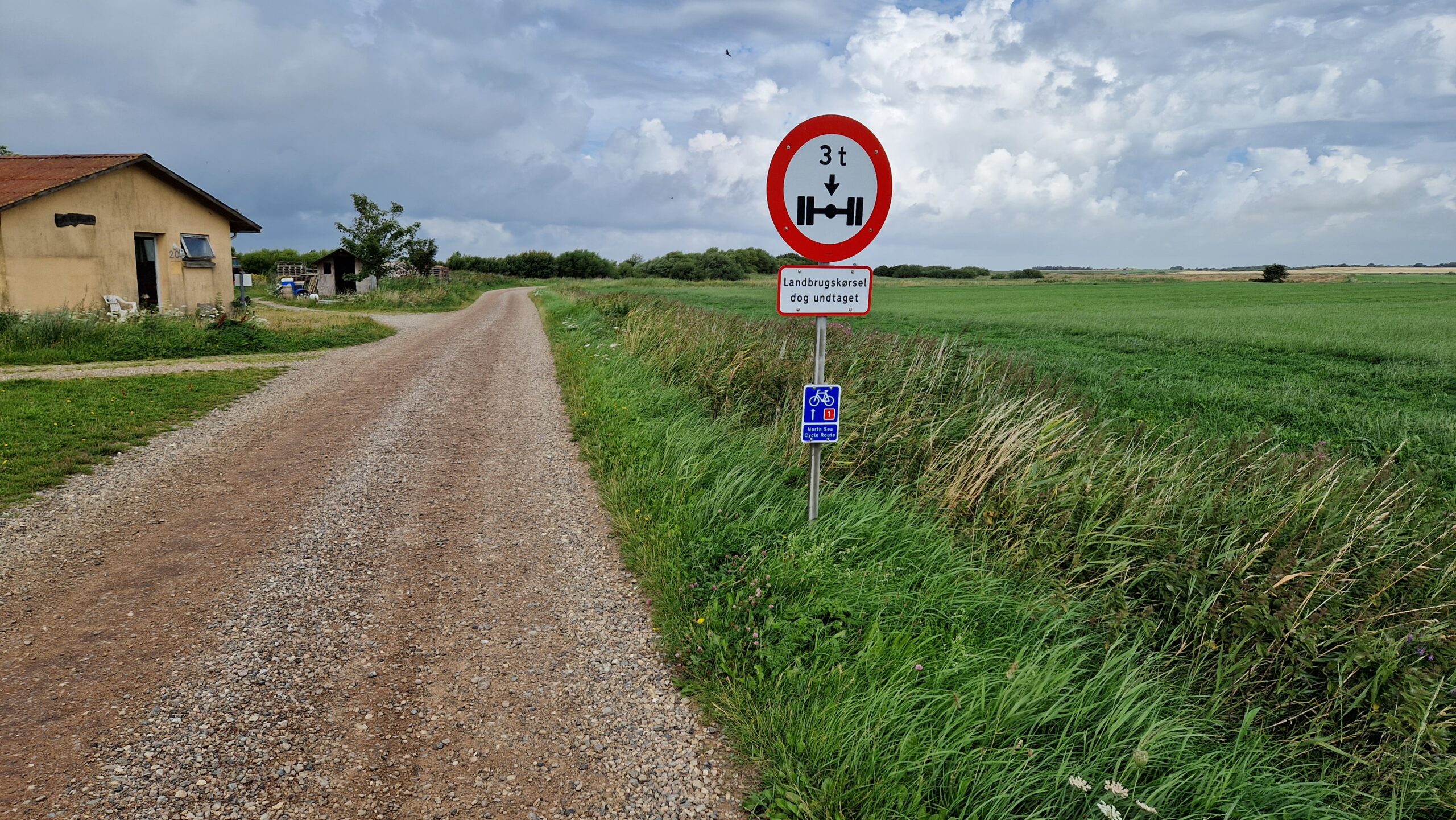
“It’s summer. Holidays. What are you going to do with your free time?” The answer to this question was quite easy: cycling! I’m still pursuing my long-term goal to cycle the North Sea cycle route R1, which is basically a 7000 km long route around the North Sea. I’ve already covered most parts of the German leg (Ostfriesland and Nordfriesland) in the years 2018 and 2019 but as we all know, COVID-19 happened in early 2020 and all travelling plans had to be cancelled and postponed.
Four years later, it was about time to continue the journey. My plan was to cycle Denmark by bike and tent. I’ve never been to Denmark before and I had no idea what to expect there. The concept of Nature Camping Sites and Shelters was very intriguing and I wanted to give it a try. Prepared a route with OpenCycleMap, packed my stuff and off I went to the island of Sylt where I ended my last bike tour in the summer of 2019.
Getting to Sylt by train…
Travelling to Sylt by train on weekend wasn’t the best idea. The route from Hamburg to Sylt was overwhelmed by tourists. The trains were mostly full, delayed and there was little to none space for cyclists. I had to skip a change in Elmshorn just because the train was hopelessly full and people were travelling like canned fish. After arriving in Sylt on the late afternoon, I had to discard my plans for the first day. I tried to find a camping site near the city of Kampen. I entered a camping site in Wenningstedt, set up my tent and after half an hour or so, I was approached by the security guy. He told me that the camping site was “full” and that I had to leave. So basically I was thrown out because I arrived too late and didn’t book my stay. I’ve never experienced this before, packed my stuff and left speechless. Since wild/stealth camping in Sylt is illegal and there is always a beach police, I was forced to sleep on a bench. This unintended situation gave me a huge pain in my back so I had to use painkillers for the next couple of days. I really disliked Sylt (even back in 2019) and just wanted to leave as quickly as possible. I won’t visit this island anymore. It’s just overcrowded, expensive (FCK KURTAXE) and you get treated like an animal. No thanks.
How to avoid Sylt’s “Kurtaxe”: just get kicked out of the camping site and sleep on a bench like a homeless person.
However, the next morning (Day 1), I cycled to the so-called Ellenbogen (“Sylt elbow”) and visited the List lighthouses and the northernmost location of Germany. The sunrise was really beautiful and rewarding. I cycled back to the List harbor and took the ferry to Havneby (Rømø, Denmark) at around 08:30. After leaving the island Rømø at around 10 o’clock, I started cycling the Route R1 on Jutland.
Welcome to the northernmost location of Germany!
Week 1 – West Coast Route R1 from Sylt/Rømø to Skagen
After leaving the island of Romo, the North Sea Cycle Route R1 starts.
Picture of the shelter Bjerregaard Havn.
Huge sculptures in Esbjerg: “Mennesket ved Havet”.
Another shelter on the beach, just outside of Fjaltring. I liked this one very much.
The cycle route leads to this section where you can cycle 3-4 km along the beach or jump into the water!
After reaching Skagen, the route leads to Grenen, the northern tip of Denmark.
360° view of the northern tip of Denmark.
This route was (officially) about 550 km long and it took me 7 days from Havneby to the northernmost location in Denmark. The west coast route was beautiful. Besides beautiful landscapes (dunes, forests, fjords, bays, sea) and mostly good to excellent cycling weather, the cycling roads were in a very good condition and also varying in quality: asphalt roads, gravel, sand/beach, forest paths, hills. I had little to no trouble with winds because the cycling routes were guarded by wind-stopping forests, dunes or dikes. 50% of the cycling time I had a weak wind, 25% back wind and 25% head wind. Day 3 was very rainy, the rain lasted for several hours but was gone in the afternoon. The route signs on the route were mostly visible, at some points they were either hidden, missing or inconclusive. This resulted in many extra kilometers because I lost track of the route. In the end, I cycled around 620 km.
Camping sites were in a good to very good condition although a bit expensive in the range from 160 to 230 DKK per night which corresponds to 23 to 32 EUR per night. It’s a bit much for cyclists with a tent if you compare it to Germany (price range from 12 EUR to 20 EUR per night). However, the shelters were free of charge so spending every second or third day on a camping site in order to get a shower and to charge up batteries was sufficient. Unfortunately, someone stole my fast charger and power bank during my stay in Ribe on Day 1. Luckily I carried a backup power bank and a charger – albeit much slower to charge – so I had to turn on the flight mode and save energy for the rest of the tour.
I met many other cyclists on route and it was an amazing experience. Everybody was friendly and supportive and we shared our cycling plans and stories. Two of those amazing cyclists were Tim from UK and Justin from Switzerland. We met on Day 3 (the rainy day) like two times on the road and later in the evening (by coincidence) in a shelter. We talked about our routes and we jokingly agreed “Our next shelter will be at X, so if you join us, it would be great to have you with us!”. The shelters were 80-100 km apart so it was quite a challenge to get there. So I cycled the next couple of days for 8 hours daily and I was able to meet them at the shelters we agreed upon. As I showed up, they couldn’t believe that I made it! Tim was very excited and sponsored me a beer on each evening. Unforgettable! We parted our ways after Day 6. Tim went on his tour to Norway and Justin continued his journey in Sweden.
Cycling from Hirtshals to Skagen was really amazing. I had about 3 hours of back wind, very good weather and great views. I took some pictures of the area although I didn’t take a walk to the Northern Beach. There were too many tourists present and I was afraid leaving my bike unattended. I noticed a high number of Tesla Electric Cars there but one car really blew my mind: I spotted a DMC DeLorean there (the car from the movie Back To The Future) which really blew my mind.
Week 2 – East Coast Route R1/R5 from Skagen to Kruså/Flensburg
Cycling on a very rainy day. This sculpture can be seen in the city of Hadsund.
You get wet. No escape from rain.
This picture was taken in Aarhus after ordering a beer in a small bar.
View on the island Funen (Fyn) and the bay.
Cycling on a very rainy day near Aabenraa.
This beer concluded the cycling route. Picture taken in Flensburg.
After reaching Skagen and the northernmost point of Denmark, I had to cycle back to Germany – a distance of approx. 620 km. Day 8 (Hulsig – Dokkedal) was a very good cycling day (111 km) with lots of interesting encounters. The following days (Day 9 and 10) were really difficult weather-wise. A bad weather zone called Hans was raging over Scandinavian countries and brought a lot of rain. The situation in Sweden and Norway was very dangerous because some local rainfalls were extreme and flushed away streets and railways. Day 9 (Dokkedal – Fjellerup) was raining the whole day. I was wet both inside and out. This was no problem because I had exchange clothes which stayed dry during the ride. Staying warm and dry during the night is much more important than during the daytime. On Day 10, the rain went away but there were strong winds at 60 km/h in combination with hills. This combination of winds and hills was very tiring and I wasn’t able to cycle large distances (55 to 65 km per day at best). Hans was almost gone on Day 11 (Balle – Aarhus) but I had to fight the terrain: hills after hills. While the West Coast Route was mostly flat and hills were an exception, the East Coast Route was dominated by hills. The hills weren’t very large (maybe 10 to 30 meters) but very frequent. I had to push my bike frequently because of my overweight and because I was carrying too much baggage with me. Nevertheless, I was able to achieve daily distances of somewhat 70 to 90 km per day which were inside of my comfort zone.
The landscape along the east coast route was dominated by cities with harbors, bays, smaller villages and agriculture. On sunny days, the landscapes were beautiful and very varied. The hills were quite a challenge which were a very nice addition to the overall cycling experience. During the last day of cycling from Fredericia to Kruså (Day 14), I was able to cycle another 109 km although the weather got really bad in the afternoon. I visited a camping site in Kruså which was about 10 km away from my destination: Flensburg.
The next day, I cycled across the Danish/German border to Flensburg, bought myself a Flensburger Pilsner beer and celebrated a successful bike tour. The travel back from Flensburg to Braunschweig by train took me another 7.5 hours.
Summary
The green marking highlights the (approximate) cycling route. I’ve cycled around 1250 km in 14 days.
I really enjoyed this adventure. My arrival day from Braunschweig to Sylt wasn’t going as planned. I had to sleep on a bench because I was thrown out from a camping site. My charger/power bank was stolen. My back/ass hurt all the time. I got lost many times and had to ride extra kilometers. I had to push my cycle and walk uphill many times… Nevertheless, a 40 year old guy weighing 120 kg (240 lbs) doing a 14 day cycling tour in a foreign country worked out pretty well! I’ve visited beautiful and interesting places and cities (Esbjerg, Hvide Sande, Hanstholm, Blokhus, Hirtshals, Skagen, Fredrikshavn, Fjellerup, Grenå, Aarhus, Juelsminde, Fredericia, Kolding, Hadersleben, Aabenraa), yet I haven’t seen them all. The holidays in Denmark were quite affordable (~500 EUR for 14 days including food and camping and 2 extra days of arrival and departure). I plan to return to Denmark maybe next year and cycle the remaining part from Fredericia via Odense to Kopenhagen.
Changes of temperature may affect measurement instruments in a negative way: thermal noise, drift of operating points, thermoelectric effect etc.. Every device has a so-called temperature coefficient (short: tempco or TC) which states how the system behaves when subjected to temperature change. Tempcos have to be taken into account when designing an electrical circuit (e. g. a voltage reference or an oscillator) or running an instrument outside of defined environmental conditions. Humidity usually affects the buildup of electrostatic charge, growth of biological organisms (e. g. mold), it may accelerate corrosion of metals and may lead to changes of electrical properties of capacitors and mechanical properties of some materials such as wood or epoxy due to surface absorption of water molecules. Therefore the environmental conditions have a significant influence on any kind of measurements and therefore need to be monitored and controlled. Since the “controlling” part (a.k.a. air conditioning) can be very difficult and expensive for a hobbyist nowadays, I was interested into the “monitoring” part.
Monitoring temperature and humidity during measurements can be of great help as soon as one has to analyze and interpret long-term measurement data. Usually the crucial question is: “Can this unwanted drift of my Device Under Test be attributed to the change of environmental conditions?”. If the answer to this question is “yes”, one can decide to take appropriate measures to deal with changing environmental conditions.
Monitoring temperature and humidity can be done very easily. Everything one needs is a sheet of paper, a pen, a clock, a thermometer and a hygrometer. Writing down time, temperature and relative humidity is the simplest method of monitoring the environmental conditions. But what happens if you have to run a measurement over a span of few days or weeks? You certainly would have to deal with missing data or data gaps. This is where a temperature and relative humidity (TH) data logger comes in place as a very useful piece of test equipment. A TH data logger is basically a small computer with storage memory (e. g. SD card), a clock and temperature/humidity sensors. Modern devices have more capabilities such as WiFi connection, graphical displays, multi-sensor logging, database connection and much more. A data logger is used to monitor environmental conditions 24/7 in a laboratory or any room of a building (bathroom, basement, radio shack, storage room, …).
Computers, memory and temperature/humidity sensors have been become very affordable in recent years and can be easily turned into loggers. This can be done with inexpensive Arduino based microcontrollers or Raspberry Pi single-board computers.
Buying stuff – the devil is in the details
Me being lazy, I didn’t want to spend much time on the development of temperature loggers. I am certain that there are few interesting projects on GitHub out there which I’ll check out soon(tm). After a few weeks of searching, I found two commercial dataloggers on Kleinanzeigen (German analogy of Craigslist) in the 60-90 EUR range which is not bad at all. One of those data loggers I acquired was the Lufft Opus 10. I’ve heard of the German company Lufft before – they are a reputable company in the fields of climate and environmental measurement equipment. Opus 10 is a TH logger with a LCD display and an USB interface for readout/control of the device. It was manufactured by Lufft in the mid 2000’s and I bought a second hand unit still in a working condition – albeit the battery was already drained up and needed to be replaced soon and it will probably need a calibration.
Lufft Opus 10 Temperature/Humidity Data Logger
As soon as I got the TH logger, I started looking online for drivers, software and documentation. I realized that this particular product was discontinued by Lufft probably 10 years ago and there was no real support for this product. Thanks to Google search and Archive.org I was able to find the manuals, datasheets and the Lufft SmartGraph logger software.
Wayback Machine from web.archive.org. This website saved my day many times. Please consider donating 😉
Lufft Opus 10 teardown and battery replacement
I’ve made some photographs of the inside. Opus 10 is measuring the temperature probably with a NTC resistor (blue blob) and the relative humidity with a capacitance sensor. Besides that, I couldn’t find anything unusual. FT232BL can be seen clearly, along with two EEPROM ICs. Off-the-shelf-components from the mid 2000 era were used, I haven’t seen any special circuits or ASICs.
Lufft Opus 10 back side
Lufft Opus 10 teardown: front
Lufft Opus 10 teardown: front detail
Lufft Opus 10 teardown: integrated circuits detail image
Lufft Opus 10 teardown: display and sensor board
Lufft Opus 10 teardown: circuit board back side
Description of the problem
After plugging in the USB device in my PC, the device couldn’t be found and drivers had to be installed manually. Unfortunately the SmartGraph software did not contain any Opus 10 drivers so no communication could be established between the data logger and PC. I thought maybe the previous versions of SmartGraph may have the drivers included so I started downloading versions dating back to the Windows 95 era. No luck at all. No drivers could be found. Since I didn’t have the original installation CD-ROM (or diskette), I could not establish a connection to my PC. It was a bit disappointing but not bad – the device would act as a TH display for the next couple of months which was good enough for my “pen-and-paper-logging” approach.
An unknown device “DATALOGGER” shows up soon after connecting the device to the PC.
Fast forward 4 months and the battery finally died. Luckily, the seller sent me replacement batteries which were rather special type 14500 batteries (Li-SOCl2, 3.6 V) – not the standard AA 1.5 V. Battery replacement was a piece of cake, no problem at all. But as soon as the unit woke up, it was asking for a “SET CLOCK” procedure. After checking the manual, I soon realized that I had a problem: after battery replacement, the internal data logger clock needs to be synchronized with the SmartGraph software. The following three days were an unique PTSD experience in combination with nightmares. Being a bit pissed off that I probably just bricked the unit by simply replacing the battery, I just thought “Fine, I’m going down this rabbit hole – should have done it four months ago” and try to fix this damn thing.
After changing the battery, the Opus 10 unit asks for clock sync. This can only be accomplished via SmartGraph software, otherwise the data logger is rendered unusable.
I don’t want to write down every step and every Trial & Error in detail. I’ll try to give the reader of this blog entry an installation procedure in a short manner so everyone using this kind of Lufft Opus Series can install the drivers and establish a connection with the PC.
Fixing the brick
During the teardown I noticed that the communication between the data logger and PC is performed via a FTDI FT232BL integrated circuit. It’s basically a USB to serial UART interface with many features, e. g. the capability to store “USB Vendor ID (VID) and Product ID (PID), Serial Number and Product Description strings in external EEPROM”. During the late 1990’s and early 2000’s, the communication of similar Opus models was usually performed via a 9-pin serial interface (also called COM-port or RS232). They must have upgraded their legacy peripherals from RS232 to USB in the early/mid 2000’s. There are probably two EEPROMs on the lower PCB: Atmel812 93C56A for sensor data and DS 2430 for USB VID/PID. I couldn’t find any microcontroller on board, since the data from the sensors need to be converted in physical units and communicated to the display. Perhaps it’s hidden under the LCD display.
Now knowing that a FT232BL integrated circuit is used inside of Opus 10 is an important bit of information because one can pin down the correct drivers provided by the manufacturer Future Technology Devices International Ltd (FTDI). Just a quick sidenote: FTDI has been confronted by plagiarism ICs in the past where their chips were copied by different Eastern Asian companies. Using a plagiarized IC with their driver can be seen as breaking the user’s license. There may be a scenario where FTDI drivers can brick a plagiarized device due to “reasons”. I haven’t observed it yet, just heard of the possibility where the drivers renders the fake IC unusable or at least it blocks its operation – so be careful and make sure you’re using the original (expensive) FTDI IC!
Installing Windows XP on IBM ThinkCentre PC in 2023. Yeah, I haven’t thought I would do it ever again but somehow it worked perfectly fine. I was lucky and kept my old software all the years!
As a side project, I digged up my old IBM ThinkCentre PC from the 2004 era and installed Windows XP on it. Sometimes it’s nice to have one old PC for testing 20 year old hardware and software. After plugging in the Opus 10 into the PC, I get an unknown device called “DATALOGGER”. I wondered why the device was called that way and where did it get its name from instead of generic name such as “USB Serial Port (COM3)”. After two days of research and trying different things out, I’ve stumbled upon the FTDI Technical Note TN_100: USB Vendor ID / Product ID Guidelines. Basically FTDI ships their ICs with default VID and PID which can be customized by anyone who’s using them in their electronic designs. So basically there is a small EEPROM chip where the “DATALOGGER” name string and the custom PID are stored. Every time the USB device is plugged in, it sends those identification strings to the PC. The PC needs to find proper USB drivers which match the VID/PID. I’ve looked into the hardware description of Opus 10 and got the VID Number 0403 and PID string “D6B8\12345678”. So they customized the PID and identification strings which was a problem for the operating system. The table below helped me to identify the VID/PID associated with the FT232BL so I started looking inside of the driver INI-files for this kind of information. I’ve quickly found the 0x0403 and 0x6001 IDs and I was hoping that renaming the default PIDs into the Lufft customized ones would help the operating system with driver identification. So that’s basically what fixed the problem. I edited bunch of INI-files and after plugging in the data logger, it was recognized immediately and I was able to install the proper FTDI drivers. The FTDI Application Note AN_107: Advanced Driver Options has a bunch of additional information how to customize their driver settings.
Excerpt from Table 3.1 from FTDI’s TN 100.
This workaround should also work on modern PCs running Windows 7 or Windows 10.
Step-by-step procedure
(Unfortunately) I am using a German version of Windows XP. However, it should be possible to get the idea of what needs to be done. After plugging in Opus 10, check the Device Manager for the newly discovered DATALOGGER. Check its properties and look for the “Hardware Detections”. There should be somewhere the VID and PID of the device. Write down the VID/PID and download the FTDI drivers for your operating system.
The Opus 10 VID/PID can be seen in the DATALOGGER properties.
I’ve been testing many versions of the FTDI drivers but it seems there is no significant difference between them. Just get one which works on your system (WinXP x32 in my case). I’ve downloaded CDM 2.08.24 drivers from the FTDI website. Unzip the drivers and you should get a similar file and folder structure as shown here.
The last FTDI driver version which supports WinXP 32bit: CDM 2.08.24.
Next step demands the editing of ftdibus.ini and ftdiport.ini files. Just use a simple text editor. Search inside of the INI files for the PID number 6001. There should be in total 3 lines where PID_6001 appears. Replace the PID number 6001 with the newly found Opus 10 PID (e. g. D6B8).
Notice: Maybe it would be better to make a copy of the line to be edited and edit leave the PID_6001 line untouched just in case you plan to connect a FT232 based IC without custom Product ID! I haven’t tested it yet but it seems like a better approach.
ftdibus.ini and ftdiport.ini need to be edited as shown in this picture.
After modifying and saving the INI files, one can proceed with the DATALOGGER driver installation. Use the Device Manager and start the driver update. The driver installation wizard should be pointed to the directory with the modified INI files.
Both INI-files need to be modified in order to be able to install FTDI drivers for the Opus 10 device called “DATALOGGER”.
Since we’ve modified the drivers, the WHQL certification fails. This can be safely ignored. After two subsequent driver installations, the devices should appear as “USB Serial Port (COM3)” and “USB Serial Converter”.
Screenshots after successful FTDI driver installation.
No further changes are needed, the COM3 settings seem to be typical at 9600 baud, 8 data bits, no parity bit, 1 stop bit (a.k.a. 9600 8N1).
Default settings after FTDI driver installation: 9600, 8N1.
The last step demands the installation of the Lufft SmartGraph software. I’ve used version 3.0 from the year 2005. A newer, modern version v3.4.5 should work, too. The data logger should be visible as a new COMx device. With SmartGraph you can change settings of the data logger such as logging intervals, min/max alerts, physical units etc. Getting familiar with SmartGraph takes a bit of time so I leave this as an exercise to the reader 😉
After successful driver installation, SmartGraph software needs to be installed
COM3 inside of SmartGraph v3.4.5 represents the newly installed Opus 10 device.
Lufft Opus 10 temperature and humidity data logger
Conclusion
I consider myself “lucky” because in hindsight, this fix was easy – but it was nowhere documented on the internet. The trial & error approach cost me about 2-3 days of fiddling but it was successful in the end. The other option would have been grim: the data logger would be rendered unusable unless doing further reverse engineering. This is so unacceptable! Reverse engineering wasn’t clearly my goal on a 20 year old device – otherwise I would have invested my time in DHT11/22 and Raspberry Pi programming. There was a discussion on a German Windows 10 forum dated back in the years 2018/2021 concerning Lufft Opus 10 driver installation problems but their posts didn’t provide any useful information except “tried this driver and it worked!”. One of the users apparently fixed the problem by using a Prolific driver which I have also tried out – without any success. I’ve even contacted Lufft’s Support on this matter and they kindly provided me some information and further hints what could be done.
For my part, I’ve learned again: The Internet DOES forget. Thanks to Archive.org it was possible to browse old websites and get documents and files which I needed. It’s very important to download drivers and documentation and host them on independent sites. Otherwise it will become even more difficult in the years to come to have access to information of already discontinued products.
I’m hoping that this information will be useful to other amateur radio operators because there are some similar problem descriptions concerning the usage of programmable transceivers. Those transceivers also use a USB/RS232 IC which demand certain FTDI drivers and perhaps it’s possible to revive them with a simple modification of the INI files.
The German Amateur Radio Club (DARC) has just recently set up their own Mastodon-based social network server. It’s basically a social network similar to Twitter with a decentralized server structure. I think I’ll try it out for the next couple of weeks and share bits and pieces of daily adventures which may not fit in a classic blog format. Currently there are 114 registered entities at DARC and perhaps more people and amateur radio districts will join.
I must admit that I strongly dislike the anti-social part of social networking which extends in the fields of politics, religion, manipulation, opinions, viral social debates and trolling. One word: internet toxicity. I like fun and memes. Let’s hope the toots stay technical and hobby-related 🙂
If you’re member of the DARC, you can set up a Mastodon account with your existing login information at https://social.darc.de
Currently I’m preparing my equipment for the next SAQ broadcast on Sunday, July 2nd 2023. There will be two transmissions: first transmission at 11:00 and second at 14:00 o’clock (CEST).
Preparing for the SAQ transmission. Some items from the junk bin.
During a flight back home from a recent business trip, I was lucky to get a window seat. I was thinking of the possibility to see some stars of the night sky above the clouds and I wasn’t disappointed. The flight was held entirely during night time with cabin lights turned off. This was crucial because cabin lights are an additional light source which make unwanted reflections visible. The reflections usually overcast faint light sources such as stars. I took some photographs with my smartphone Samsung Galaxy S22 at exposure duration of 20-30 seconds and ISO 3200. The exact location of the photograph is unknown, it must have been somewhere in a part of south-eastern Algeria over the Sahara desert while looking to the east. I would estimate the position as follows: 23° North, 8° East, flight attitude 11 km (36 000 ft).
Result of a shaky picture during long exposure duration (20 – 30 seconds). The stars appear “smeared”
I made about a dozen pictures of the night sky but due to minor turbulence and slight flight course corrections, most of the images were shaky and had to be discarded. However, I was able to get 1-2 pretty decent pictures of the night sky which turned out to be OK. I was pressing my smartphone against the window to avoid shaking motion and put a pillow over it to block most of the residual (emergency) cabin lights.
Beautiful night sky picture taken with a smartphone from an airplane window. 20 second exposure at ISO 3200
The taken pictures show some prominent stars from the constellations Cygnus and Lyra: Vega, Deneb, Albireo and others. I was able to identify some stars by using an web-based star map application such as Stellarium Web. During the flight I could observe meteor flashes occasionally (no picture taken though) and lightning of distant thunderstorms, which were perhaps >200 km away. There were virtually no city lights visible during the flight over Sahara desert. Just imagine being there and watching the night sky without any light pollution…
Identified stars from the constellations Cygnus and Lyra
Stellarium Web
The 8-hour-flight was very tiring because of lack of space to move and stretch. Sitting for hours in an uncomfortable position wasn’t very pleasant but it worked out somehiw. However, I was able to catch some nice pictures of the world 11 km below my feet. #worthit
Rising sun and parts of the night sky
City lights from Khenchela, Algeria
Picture of Genua, Italy
Skyline and Football Stadion from Frankfurt/Main, Germany
Measuring voltages accurately is a basic task for technicians, engineers and scientists. The voltages to be measured range from perhaps few picovolts to several megavolts – a dynamic range of 18 orders of magnitude! But every modern digital multimeter is kinda limited in resolution. The multimeter’s resolution can be stated in the number of digits it can resolve. A 6 digit multimeter can resolve six decimal places going from 0 to 9. In a decimal number system, this corresponds to \(10^6\) numbers or 1 million digitizing steps. Without going much into detail and exposing my limited knowledge on this matter, I’ll just link to Keysight’s Website where everything is well explained.
Older multimeter models such as the shown MeraTronik V543 can resolve only \(2 \cdot 10^4\) numbers in the selected measurement range (e. g. ±1 V = 2 V full scale: \(2~V/2 \cdot 10^4 \rightarrow 100~µV\) resolution).
MeraTronik Type V543 (PRL T-189), 4.5 digit multimeter with Nixie tube display
One of the best and most accurate digital multimeters in present time – the HP 3458A – has “only” a resolution of 8.5 digits, which hasn’t improved for about 35 years.
HP/Agilent/Keysight 3458A 8.5 digit multimeter
The so-called “Voltnuts” (crazy electro-fanatics) buy those HP multimeters on a second hand market for $3k to $7k. This surely is crazy and overpriced and in my opinion just not worth it. How about buying a couple of cheaper 6.5 digit multimeters (e. g. HP 34401A for about $200 to $400) and combining them in a serial configuration? I’ve achieved a total of 19.5 digit resolution this way*. I was able to display 10 volts up to 18 decimal places, e. g. attovolts resolution and saved a lot of money.
Two HP/Agilent/Keysight 34401A 6.5 digit multimeters in an unusual configuration showing exactly 10 Volts on April 1st…
*If you don’t believe this nonsense, it’s fine. I can live with that. It’s April Fools’ day anyway 😉
About a year ago I saw one of CuriousMarc’s YouTube videos on repairing a Xerox Alto computer. CuriousMarc published shortly afterwards an episode, which compared the Tauntek LogICTester with the TL866II+ EEPROM programmer which has some transistor-transistor logic (TTL) testing capabilities. 1970’s and 1980’s era test equipment used alot of those intergrated circuits (IC) in order to operate. Servicing or repair of older test equipment like oscilloscopes, multifunction calibrators, power supplies etc. will be much easier with tools such as a logic tester. After reading a very positive review from a friend at the Wellenkino, I thought it would be very nice to own such a tester for servicing or repairing my (broken) equipment.
Tauntek LogIC Tester
I contacted Bob Grieb of Tauntek and ordered one of his kits back in March 2022. The $35 kit contained the printed circuit board and two pre-programmed PIC microcontrollers. The shipment to Germany cost me about $19 with additional 10 EUR for customs and fees. The total cost for the kit ans shipment was in the order of $64 or approx. 60 EUR. The shipment from USA to Germany took about week and a half.
Shipment received from Bob Grieb of Tauntek.
After receiving Bob’s package, the project got delayed because I’m always kinda busy. I ordered most of the remaining parts via Mouser in December 2022. The ordered parts would cost additional 69 EUR. Many of the components on the bill of materials (BOM) list could have been easily skipped (e. g. resistors and 2x PIC microcontrollers, RS232 level shifter) resulting in 45…48 EUR price range. Nevertheless, I ordered few extra parts just to be sure if anything fails. Extra parts can be always used for different projects or experimenting with other circuits.
Two of needed parts on the BOM weren’t available at the time: the 74HC138 3-to-8 line decoder and LM358AN dual opamp. According to Mouser, the lead times for the decoder were four weeks and for the opamp approx. 1 year (which has been reduced to May 2023 in the meanwhile). So yeah, I had to order both parts on eBay instead. Waiting a year for an opamp wasn’t acceptable. I also ordered an USB to TTL FTDI Serial Adapter on Amazon (2 pieces for 8 EUR) so I could use the Tauntek LogICTester via USB instead of RS232. Everything arrived last week so I had to find few “quiet hours” for the soldering job.
Building the IC Tester
One starts with the printed circuit board and two PIC microcontrollers (U1 as Master and U2 as Slave) as shown in the picture below.
The unboxed Tauntek LogICTester.
I started populating the resistors and diodes in the first place. After soldering and cutting excess wires, I moved on to capacitors.
Starting the population with passive components is always a good idea….
Population continues, only few more parts…
Chaos unfolds when doing a soldering project…
After hours and hours, I finally got it finished. The pins in the top right corner needed to be removed. Also JP1 and JP2 (top right above the IC socket) were shorted by a solder blob in order to use the FTDI to USB adapter instead of the RS232 level shifter. The level shifter 16 pin socket on the top right remains unpopulated. The final assembly can be seen in the picture below.
After assembly I checked for cold joints or shorts. Everything looked fine and I turned it on.
Tauntek LogIC Tester: finally assembled and ready for IC testing.
After plugging in the USB cable of the FTDI adapter into the Windows 10 machine, the driver installation started automatically. No additional drivers were needed to be installed. The settings for communication via Serial connection were by default “8-N-1”, which corresponds to 9600 baud, 8 data bits, no parity bit, 1 stop bit and no flow control. The connection needs to be established via a terminal emulator such as PuTTY. After establishing a connecting to the tester, one has to press ENTER to get the welcome screen and voilà, We’re In Like Flynn.
The usage of the IC tester is pretty much straight-forward. Power up the tester, establish a PC connection and put the IC into the socket as shown in the picture above. Enter the IC model inside of the console. If the IC is found inside of the database, type t and press enter to start the IC test. The results are presented in a very comprehensive way. Typing v and pressing enter displays the pin voltages.
Tauntek LogICTester menu via terminal emulator PuTTY.
That’s it – there isn’t much more to it. Very simple and effective when it comes to debugging the 1970s to 1980s era logic ICs. Few additional hints and comments:
Unfortunately the IC tester can not be used in order to recognize part numbers of ICs under test. The part numbers have to be looked up manually inside of the terminal emulator (or Bob’s list)
Bob maintains the firmware and the list of supported ICs. Perhaps by writing him an email and by sending him the missing or unsupported IC, Bob may update his firmware in the future and add support for the missing IC
The logic tester certainly isn’t free of bugs – some tests may result in a “FAIL” although the IC is still fine according to the datasheet specifications. Please, don’t blindly trust the machine. Take your time and try to sanity-check or interpret the results
If one wants to capture analog images or analog videos (e. g. images coming from a CCTV camera), those signals need to be digitized, decoded and displayed with a device called framegrabber. A framegrabber is basically a video capture card with fast video processing capabilities and onboard memory which is useful for image processing.
I wrote in my previous post how to make good quality screenshots of the Anritsu MS2661N front display. However, there is another ancient method how to acquire images of frequency spectra. In modern test equipment, the video signals are transmitted digitally via DisplayPort or HDMI. Some 20 to 40 years ago, the manufacturers offered instruments with an optional analog video output which could be connected to a television screen or to a video recorder for viewing or documentation purposes.
75 Ohm composite output can be seen on the back side of the Anritsu MS2661N spectrum analyzer
I’ve got myself a framegrabber card NI PCI-1405 for different projects. I wanted to test the card for its functionality. The quickest access to an analog video was via the composite output of my spectrum analyzer as shown in the previous picture.
NI PCI-1405 Video Framegrabber Card
The NI PCI-1405 framegrabber card has two inputs: a 75 Ohm video input and a 75 Ohm trigger. The video input is connected via a 75 Ohm cable (type RG-59) to the composite output of the spectrum analyzer.
The 75 Ohm coaxial cable (RG-59) needs to be connected to the video input of the framegrabber card
After installing the drivers from National Instruments, the framegrabber card was successfully detected and I was able to grab some frames inside of NI MAX (Measurement & Automation Explorer).
Framegrabber user interface inside of NI MAX
I didn’t bother to improve the image quality – this task will be relevant for future projects as soon as I get my Tektronix C1001 camera running 🙂 So far, it’s been a successful test!
Grabbed frame in a 640×480 resolution. The analog source signal was received in greyscale NTSC format at approx. 30 frames per second
Tektronix 2456B with attached Tektronix C1001 video camera