Tektronix

Tektronix TDS 3034B bandwidth upgrade

Tektronix TDS 3034B four channel color digital phosphor oscilloscope.

A “new” oscilloscope arrived in the lab just recently thanks to my friend Matt, who relayed the offer to me. It’s a wonderful instrument from the early 2000’s era: a Tektronix TDS 3034B Four Channel Color Digital Phosphor Oscilloscope. The oscilloscope’s analog bandwidth is specified at 300 MHz with a sample rate of 2.5 GS/s per each channel. It has a ton of options (e. g. FFT, 3LIM, 3TRG) and a communication module with VGA monitor output and GPIB/Ethernet/RS-232 for communication and control. There is also a battery compartment, however, the battery was not included. The “Waveform Intensity” knob simulates the intensity control of an analog oscilloscope with a cathode ray tube – therefore a “Digital Phosphor Oscilloscope” or DPO. The size of the oscilloscope is very convenient and perfect for a desk use – doesn’t take much space and it’s fast and responsive compared to my older Tektronix TDS 754D oscilloscope.

Tektronix TDS 3034B back side with battery/probe compartment.

I was able to set up the communication to my PC via GPIB (IEEE 488). Since I already had the Tektronix WaveStar Software for Oscilloscopes installed on my Windows 10 PC, I was able to quickly transfer screenshots/hardcopies, measurement data and sample data from the instrument to my PC. No diskettes or USB drives were needed. It is possible to control the oscilloscope remotely which is absolutely fantastic for measurement documentation and measurement automation purposes! It’s a great addition to the lab and it will serve to me as my daily workhorse among other oscilloscopes, of course.

Tektronix WaveStar for Oscilloscopes. Easy way to transfer screenshots and data from Tek TDS 3034B to a Windows PC.

Bandwidth Upgrade

It seems to be very common (even nowadays in 2024) that the oscilloscope manufacturers design a generic oscilloscope parts which can be used for different models. The oscilloscopes are then assembled with similar to identical hardware components (presumably because it’s cheaper manufacturing-wise) but the measurement capabilities are determined either by hardware (jumper settings) or by software (locked/unlocked options).  For example, Rigol DHO 800/900 Series Oscilloscopes can be upgraded from 70 MHz to 100+ MHz via software. Thanks to Matt, he gave me a hint that the guys at EEVblog have figured out how to perform an upgrade of the Tektronix TDS Series oscilloscopes to different models. So already having an excellent 300 MHz & 2.5 GS/s oscilloscope at my fingertips, I was curious if I could upgrade it to the 3064B model which has 600 MHz analog bandwidth and 5 GS/s sample rate. I tried out the EEVblog’s upgrade procedure and it seemed to work without bricking the oscilloscope. I’ll just quickly summarize the procedure here.

  • Boot up the device and set up the communication via GPIB (e. g. GPIB address and talker/listener mode). Connect the device to your GPIB controller
  • I used the National Instruments GPIB-USB-HS controller device along with current NI’s GPIB drivers (driver version doesn’t matter much, you could also use the VISA drivers from Keysight, Tektronix or Keithley). The TDS 3034B Firmware Version was v3.39
  • The communication between the PC and the oscilloscope was established with NI Measurement & Automation eXplorer’s (NI MAX) own GPIB Instrument Communication. I guess you could use any GPIB communication software, e. g. pyvisa for Python
  • Check whether the oscilloscope responds to the *IDN? query. If yes, proceed, if not – try to find the problem and fix it (obviously)
  • Send the following commands to the oscilloscope
    PASSWORD PITBULL
    MCONFIG TDS3064B
    Just send (write) the commands in the order as shown above! Do not use a “GPIB query” since there will be no response action from the oscilloscope. Upper/lower case letters don’t matter.
  • Now power-cycle the oscilloscope (turn it off, wait few seconds and turn it on again). It should boot up with a new screen and new model. If it doesn’t show the new model, something went wrong with command transmission via GPIB. As far as I could tell, some models accept only different MCONFIG-commands, such as “MCONFIG TDS3054” without the letter “B” at the end. Anyways, after sending the commands via GPIB and power-cycling the oscilloscope, it should show up with the new model
  • Changing the TDS model will result in an uncompensated waveform. I observed a DC offset and noise on my CH1 through CH4 waveforms post-update. The solution to this problem is quite easy: wait some time (at least 10-15 minutes) for a warm-up and perform the Signal Path Compensation (SPC), which can be found in the Utility → System Config → Cal
    menu. This will perform an internal calibration where the noise and offset errors are compensated. The oscilloscope should be ready for performing measurements afterwards

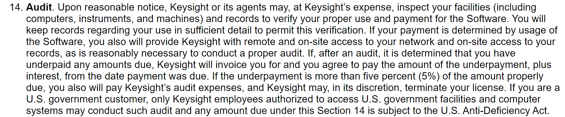
That’s how it worked out for me. It took me just few minutes to convert a Tektronix TDS 3034B into a TDS 3064B. I’d recommend to check out the linked EEVblog thread for further information on the TDS 1000/2000/3000 Series upgrades. Of course I can’t be held responsible if you try it out and damage your instrument (e. g. calibration data or warranty is lost or the device is bricked) since I’m sharing this information and tried it out on my own oscilloscope. This is solely done at one’s own risk! Please be careful when trying out this procedure and please read the EEVblog thread prior to changing the instrument. Always make backups of your oscilloscope firmware prior to changes. Also hacking the device in order to use unlicensed software options is… well… “illegal”… I guess… Keysight’s Agents will hunt your PC down! 😉

Excerpt taken from the Keysight N1500A EULA. This is not a joke (well, it’s a well-known meme), see it for yourself: https://helpfiles.keysight.com/csg/N1500A/License_Agreement.htm

Checking the Oscilloscope Analog Channel Bandwidth

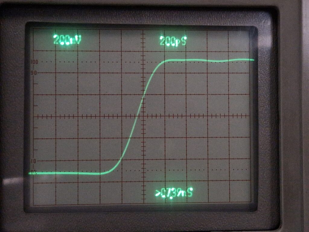
I did some initial bandwidth testing with my Leo Bodnar Fast Risetime Pulse Generator. The pulser generates repetitive 10 MHz square waves (~1 Vpp) with a rise time of around (30 ± 2) ps. It can be used to easily test the oscilloscope’s analog channel input bandwidth. The analog bandwidth of an oscilloscope can be calculated as follows:

\( \mathrm{BW [GHz]} \approx \cfrac{0.35}{t_r ~\mathrm{[ns]} } \)

So a measured 10%-90% rise time of \(t_r = 1.000 ~\mathrm{ns}\) results in an analog bandwidth of \(0.35/(1.000 \cdot 10^{-9} ~\mathrm{s}) \approx 0.350 \cdot 10^9 ~\mathrm{Hz}\) or 0.35 GHz which is basically 350 MHz. So prior to the bandwidth upgrade we were expecting an oscilloscope bandwidth of ~300 MHz at a 2.5 GS/s sample rate, post-upgrade it should be around ~600 MHz and a 5 GS/s sample rate. I’ve measured the rise time of all four channels in order to see if there are any significant differences between them. The oscilloscope settings were as follows: Coupling: DC, Termination: 50 Ω, Trigger: External, Acquisition Mode: 64× average per acquisition at 10k points and 5.00 GS/s. The trigger was delayed by approx. -10 ns.

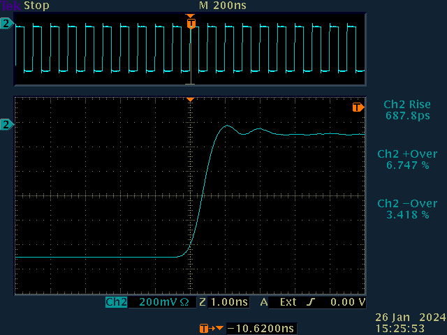
The measurement results are summarized in the table below.

Analog bandwidth calculations from measured rise times for each oscilloscope channel. Comparison between Tektronix TDS 3034B before model upgrade and after model upgrade to TDS 3064B.

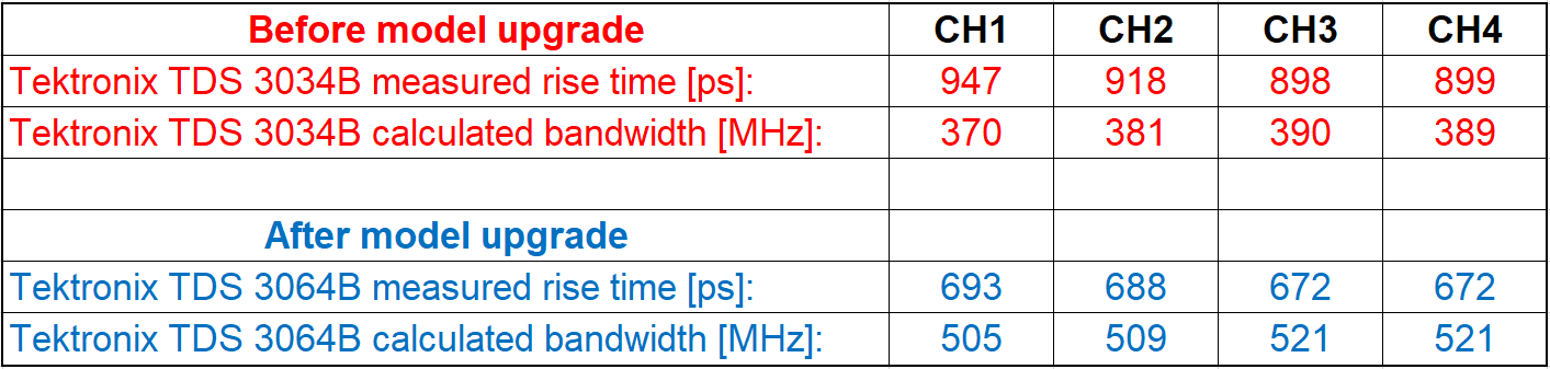
As we can see, the full bandwidth of 600 MHz for a Tektronix TDS 3064B has not been achieved. However, there is a measurable improvement. Channels 3 and 4 seem to have a slightly higher bandwidth than channels 1 and 2. The rise time measurements deviate on each acquisition so I would estimate an uncertainty in the rise time measurements of approx. ±10 ps. I also wonder if the overshoot/undershoot calculations are correct. I’ll have to look into this manually, since the data samples can be exported in a CSV file.

Conclusion

Nevertheless, the bandwidth upgrade was successful! 500 MHz analog bandwidth at 5 GS/s is more than enough for my needs before stepping into the GHz time domain regime. And no need for a battery if there is a food compartment in your oscilloscope! Tested successfully with carrots! 😉

Tektronix TDS 3034B food compartment.

Tektronix TDS 3034B bandwidth upgrade Read More »

Tektronix 7104 – 1 GHz analog oscilloscope

I’m really happy of being a new owner of a Tektronix 7104 oscilloscope – one of the fastest analog oscilloscopes made by man.

Tektronix 7104
Tektronix 7104, 1 GHz analog oscilloscope
Last time I saw one of those on eBay, I was hesitating to buy it and it went away for dirt cheap. Anyways, I didn’t want to miss a chance this time. The unit is working and in a very good condition. The horizontal and vertical plug-ins delivered with the scope are meant for the full bandwidth of 1 GHz.

The Microchannel Plate CRT display is still in a good shape – no burn-ins except the typical wear-out areas (horizontal trace, annotation areas).

Measured rise time of Tektronix 7104 with Leo Bodnar pulse generator on a 7A29 single channel vertical amplifier plugin: approx. 300 ps
Sine wave at 1.0 GHz, approx. -13 dBm into 50 Ohm

Bandwidth test with Leo Bodnar pulser on one of the 7A29 plug-ins gave me a rise time of 300 ps with an estimated bandwidth of approx. 1.16 GHz. This is my fastest oscilloscope now. I’ll check the innards in a couple of weeks.

Tektronix 7104 – 1 GHz analog oscilloscope Read More »

More Tektronix Oscilloscopes in 2022

About 2 weeks ago I traveled through the country in order to pick up – as one may guess – another Tektronix oscilloscope! Who would have thought? This unit was very special: a Tek 7904A with many high-speed plugins such as 7A19, 7A24, 7B92A… just to name a few.

The seller was very kind and showed me more stuff laying around in the basement. There were some vintage instruments on a dusty shelf but the Tektronix R556 dual-beam oscilloscopes really caught my eye. We discussed about the future of some of the test equipment and we agreed to “dispose” it the “proper” way: load it in my car and drive it to a place where it will be treated with love and respect… my apartment! 😉

20220515_153643.jpg
Those are beefy and heavy… boat anchors… err oscilloscopes 😉

I’m a TEA with somewhat heavy GAS, that’s for sure. But I have never possessed anything like a Tektronix 556 dual beam oscilloscope. Two of them. It was very difficult to carry them around because of its mass of approx. 30 kg per unit. 

20220527_141549.jpg

Nevertheless, the units made it to my home without problem. Initial visual inspection showed a somewhat pristine condition! Besides dust, all vacuum tubes were present and all knobs/plugins/parts were without any visible damage.

20220527_141110.jpg
Side view of Tektronix R556 Dual-Beam oscilloscope. Amazing piece of late 1960’s/early 1970’s technology!

I was lucky to get two fitting bezels from Matt@Wellenkino and a proper AC power cord from eBay (type NEMA 5-15R). I’ll have to wait with power-up until order has been restored in my apartment. 😉

IMG-20220516-WA0012.jpeg
The back side of the Tek R556 oscilloscope. It has a standard NEMA 5-15 AC power plug.
20220527_141359.jpg
Receptacle of a NEMA 5-15R cable.
20220527_141516.jpg
Waiting for power-up! I’ll have to check the unit first and replace old and leaky electrolytic capacitors before powering this unit up.


More Tektronix Oscilloscopes in 2022 Read More »

New Addition to the Lab: NanoVNA V2 Plus4

While browsing the Internet, I stumbled here and there upon a nice little gadget for ham radio amateurs called NanoVNA. This is a compact Vector Network Analyzer (VNA) — a piece of test equipment which allows to measure radio frequency (RF) properties of a Device Under Test (DUT) such as Magnitude and Phase. This is very useful in order to characterize RF components such as antennas, filters, cables or amplifiers – the usual ham radio stuff. Few weeks ago I ordered a NanoVNA in order to perform simple tests on my RF equipment. This article will be about  a quick set up of NanoVNA and doing some simple measurements.

Prices for “Maker/hobbyist level” VNAs  vary from 50ish EUR to ~550 EUR (DG8SAQ VNWA V3) depending on model and additional accessories. More sophisticated vintage test equipment (HP/Agilent, Rohde&Schwarz) may be found on eBay in the range from 1k+ EUR to ~3.5k EUR. Brand new entry level VNAs start at ~2k EUR without upper price limit,  depending on its measurement capabilities. As soon as you buy a VNA you will also need accessories such as torque wrench, lots of adapters (Type N to SMA to BNC and vice versa) and calibration standards (short/open/load/through, SOLT) in order to perform correct measurements. Professional calibration standards (e. g. metrology grade SOLT) are extremely expensive (~3…10k USD) and unaffordable for the low budget hobbyist – so yeah…

I didn’t want to spend 500+ EUR for a piece of test equipment which may result in even greater financial commitment. Based on the positive reviews and my requirements (easy to use, convincing measurements), I bought the NanoVNA V2 Plus4. It’s a compact 2-port VNA with integrated 4″ touch screen display, the specifications are listed here. The total price was ~215 EUR for NanoVNA + shipment + customs. The delivery from China to Germany took approx. 3 weeks from November till December 2021 (standard shipment, no express parcel).

The accessories are shown in the picture above: NanoVNA V2 Plus4 enclosed in a metal housing, two SMA cables, SOLT calibration set, USB cable and a small stylus for the 4″ touch screen. A 4/3 A type 18650 rechargeable Li-Ion battery was not provided due to transport restrictions of hazardous materials (exploding Li-Ion batteries on aircrafts…). The rechargeable battery had to be bought separately (+13 EUR). I’ve added few pictures of my NanoVNA V2 Plus4 here.

The usage of the VNA is pretty much straight-forward: turn it on, set sweep parameters, perform SOLT calibration and test your DUT. The basic measurement results provided by a VNA are Magnitude and Phase over the set frequency range. Those measurements are used to calculate very useful quantities such as  VSWR (voltage standing wave ratio), ESR (equivalent series resistance), LCR (inductance, capacitance, resistance) and plotting a Smith chart. The result can be seen directly on the 4″ display and read by different cursors. This is a perfect tool to do quick performance or sanity checks on RF components.

As soon as one wants to do systematic measurements on different components, it becomes a little bit inconvenient to photograph the Smith chart due to glare, mirror reflections and possible motion blur while taking photographs. However, it is possible to control the NanoVNA via USB and read out the measurements to the PC. The readouts can be stored and processed via standard software such as MS Excel, LibreOffice Calc, Python/matplotlib, MATLAB, GNU Octave and others. This is where the fun begins.

NanoVNA readout via USB

An user from the EEVBlog (joeqsmith) tested early versions of NanoVNA and was quite unhappy with the provided tools at the time. He developed a very useful software front end for the NanoVNA which is based on LabVIEW 2011. In his software, commands are sent via USB protocol to the NanoVNA in order to set measurement parameters and to perform SOLT-calibrations. After triggering the measurement, the data is transferred to to PC and displayed graphically and processed through math equations. He put a lot of effort in the development and the results are astonishing. His software is capable of controlling NanoVNA via comprehensible user interface, taking measurements, performing calibrations, calculating almost all imaginable RF quantities in time and frequency domain. This is very helpful for newbies like me who have never worked with a VNA before. His software can be found on GitHub, downloaded and used freely with no limitations or charge. Props to joeqsmith — he maintains an active and educational YouTube channel so check it out if you’re interested in RF or handheld Digital Multimeter testing methods.

First steps

Buy NanoVNA, plug in the USB cable and turn it on. If you’re using Windows 10, the device should be recognized as USB CDC (Communications Device Class) on a virtual serial port (e. g. COM6). Next steps will be a little bit annoying: create an account on the National Instruments (NI) homepage, download and install the NI LabVIEW Runtime Engine (Version 2011 SP1 32-bit, size ca. 215 MB) and NI VISA. I have installed VISA v17.0 which is a 750 MB chonker.  It contains drivers for USB/Serial communications any many others (also some important drivers for my obsolete GPIB test equipment which aren’t supported in the newer versions anymore). Install VISA and the Runtime Engine and spend your precious life with many reboots. I highly recommend to read Joe Smith’s User Manual, otherwise you may run into problems. Unfortunately, NI software is closed source/BLOB but everybody is encouraged to develop his own  free and open source software for NanoVNA.

After the Installation is complete, download, extract and run the Runtime Version Executable (NanoVNA_V2Plus.exe) from Joe’s GitHub. Execute the File (abort the file dialogue if you don’t have any stored calibration files) and you should see something similar to the screenshots below. Setup the connection parameters (COM-port) and establish a link to your NanoVNA.

After starting NanoVNA V2+4, one needs to select the proper COM Port. Switch to “Main” tab afterwards.

Click on the “Link” button and your NanoVNA should display “USB Mode”. The NanoVNA identifier message should appear.

Photograph of the NanoVNA V2 Plus4 in the USB Mode.

Start the sweep by clicking on the “Sweep” button. One should see some activity during the sweeps. I’ve connected a 50 Ohm load on Port 1 as seen in the Smith chart.

Alright, now we’re ready to go. Next step: SOL(T) calibration, taking measurements and data analysis. The usage of this software is described in Joe Smith’s User Manual or on his YouTube channel. He has a plenty of demonstration videos how to make proper measurements with NanoVNA V2 Plus4. This is easily done by clicking on the “2PortCal” button followed by some dialogues. After the SOLT calibration is performed, it can be saved and reused. A calibration is necessary as soon as the frequency span changes.

Sanity Tests

It’s a good practice to somehow validate your measurements. This requires some additional gadgets like filters or self-made circuits. I’ll gather some over time. I’m currently checking if the attached SOL standards are displayed correctly.

Testing a coaxial cable

50 Ohm coaxial cables such as RG58 or RG174 are widely used as transmission lines for radio frequency signals. Some important electrical properties of this cable type are: characteristic impedance (typical 50 ± 2 Ohm), capacitance per unit of length (96 pF/m), attenuation per unit of length (0.67 dB/m) and its operating frequency range (DC – 1 GHz). Data taken from Radiall’s RF and Microwave assemblies. For amateur radio operators, the SWR (standing wave ratio) is another important quantity which determines the match between impedances of the source (e. g. transmitter) and the load (e. g. an antenna). In case of an impedance match Z = Z_0, we obtain a SWR close to 1:1. We can measure the impedance Z with a little help of a VNA over a wide frequency range.

NanoVNA measurement setup. DUT: Tektronix 012-0482-00 Precision Coaxial cable. Inside of the cable loop are my BNC “calibration standards”.

This is what the measurement setup looks like. I’ve connected the NanoVNA ports to two SMA cables (blue) in order to perform a SOLT calibration. My DUT will be a Tektronix 012-0482-00 Precision Coaxial Cable which has a length of 36″ and an impedance very close to 50 Ohm. I’ll set up the measurement for 1 MHz to 300 MHz and check the SWR, attenuation/losses and its impedance. The measurement results can be seen in the figures below.

Measurement result: Smith Chart. Comparison between two coaxial cables of slightly different lengths. Frequency range: 1 MHz to 300 MHz.

Measurement result: Transmission Rectangular. Comparison between two coaxial cables of slightly different lengths. Frequency range: 1 MHz to 300 MHz.

Measurement result: Standing Wave Ratio (SWR). Comparison between two coaxial cables of slightly different lengths. Frequency range: 1 MHz to 300 MHz.

Measurement result: Reflection Coefficient. Comparison between two coaxial cables of slightly different lengths. Frequency range: 1 MHz to 300 MHz.

Measurement result: Impedance Rectangular. Comparison between two coaxial cables of slightly different lengths. Frequency range: 1 MHz to 300 MHz.

Conclusions

There you have it! Both cables show a similar performance. Tektronix 012-0482-00 shows an impedance slightly closer to 50 Ohms and a slightly better transmission compared to a no-name brand RG58 C/U. Well, maybe the sharp drop of the reflection coefficient coincides with the fact, that this cable has to be used along with Tektronix SG 503 Levelled Sine Wave Generator in order to perform oscilloscope bandwidth checks. Tek SG503  covers the frequency band from 250 kHz up to 250 MHz. Very interesting! Maybe this information may be useful to other Tektronix users. I’ll try to characterize the Tektronix coaxial cable with a “slightly better equipment” later this year, just to validate the NanoVNA measurements. Please take the provided information “as is”. It might be wrong after all.

NanoVNA – would recommend

The NanoVNA is a very useful, nice and affordable addition to a hobbyist electronics lab. Using Joe Smith’s NanoVNA software works pretty well and offers a rich repertoire of calculations and graphical diagrams. I didn’t experience any kinds problems on my Windows 10 machine while using Joe’s software. The installation and setup was straightforward and I was able to obtain plausible measurements. Unfortunately I don’t have coaxial cables with matching lengths in order to make comparison measurements with my Tektronix 012-0482-00 but that’s the part where one starts going down the RF rabbit hole…

Few things to consider

Please be aware that the components used in combination with NanoVNA are very cheap. The quality is “OK” or let’s put it in another way: “good enough for the job”. The devil is in the details. In order to perform reliable and comparable measurements, one needs quality cables, good connectors, good adapters, better calibration standards and a torque wrench. If you’re possessing good RF gear, please be careful when interchanging the components. It’s very easy to damage quality gear with cheap rubbish. I’m trying to maintain two ecosystems: the cheap components will be used for non-critical projects and quick and dirty measurements. The quality equipment will be used for careful measurements and calibration.

Going down the RF rabbit hole?

What if one already possesses quality accessories — a question might arise why not spending money on a good vintage VNA anyway? Unfortunately I’m not an RF engineer and I don’t test or develop commercial RF circuits. RF is just a hobby and not my daily business. This kind of affordable tool lets you make a first step into the world of RF components and circuit testing. I don’t need to emphasize its usefulness for testing and debugging of RF circuits or performing sanity checks. I’ll keep looking for a vintage HP/R&S VNA because the answer to this question is always YES.

73 de DH7DN

New Addition to the Lab: NanoVNA V2 Plus4 Read More »