Anritsu MS2661N Spectrum Analyzer Readout
Introduction
A spectrum analyzer (SA) is a very useful tool when it comes to measure spectra of radio frequency signals. I recently acquired a 2004 era spectrum analyzer. It’s from a Japanese test equipment manufacturer Anritsu and the model number is MS2661N. Luckily there are operating manuals available online but I wasn’t able to find service manuals for this type of spectrum analyzer on the internet. There are some service manuals available for similar models of spectrum analyzers (e. g. MS2650/MS2660) which would allow troubleshooting but I would be lost if the instrument breaks.

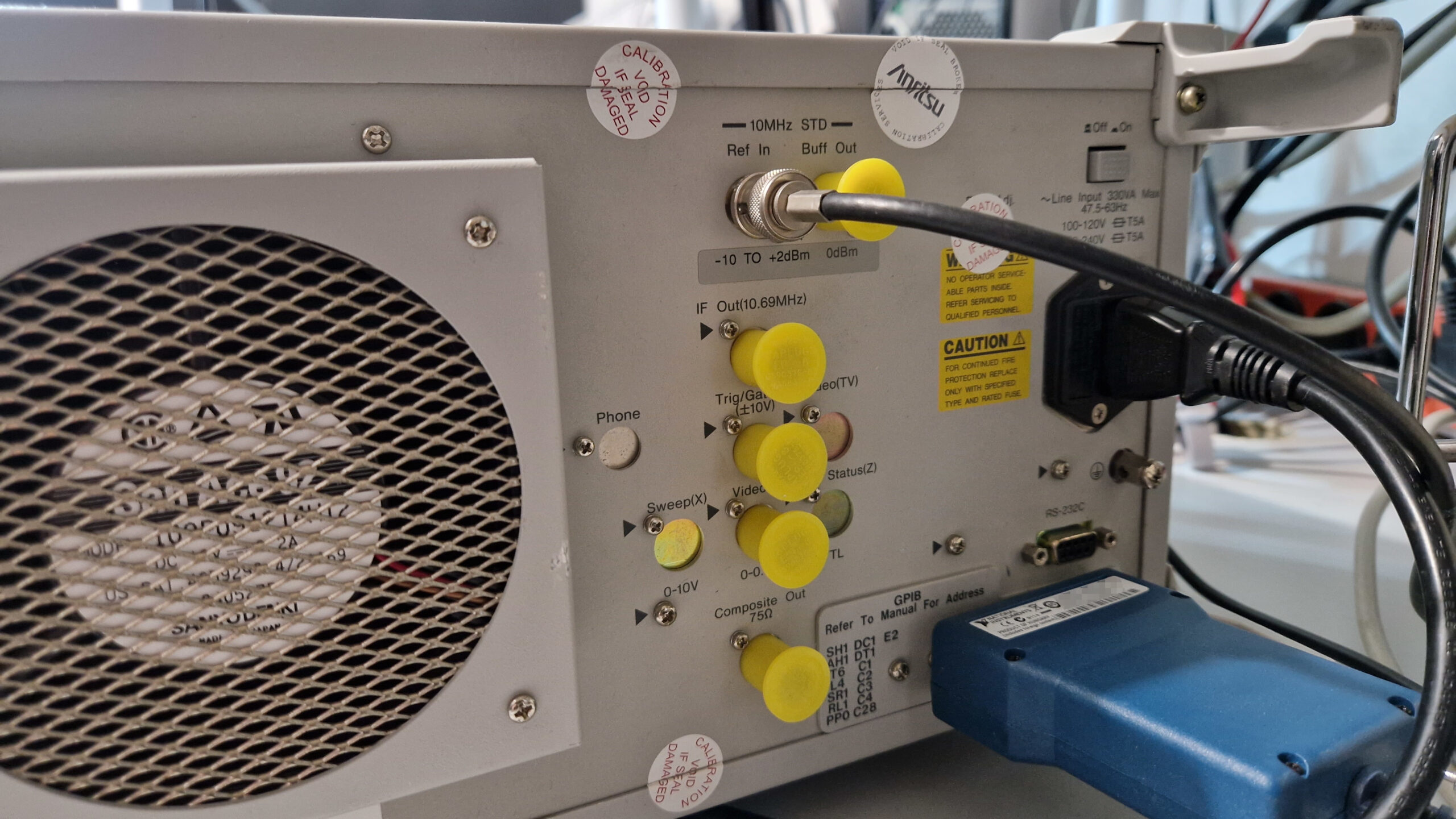
However, I’ve been looking for a decent SA for a longer time and stumbled upon the Anritsu MS2661N. It had a bunch of very nice and useful features: frequency range 100 Hz to 3 GHz, 30 Hz resolution and video bandwidth, oven controlled crystal oscillator (OCXO), GPIB interface, 10 MHz reference IN/OUT and a tracking generator ranging from 9 kHz to 3 GHz. I was looking for a similar SA from HP/Agilent 8590 Series or Tektronix but there were no attractive offers at the time. Either the SA frequency range was too low for modern ages (1 GHz) or outside of my measurement capabilities (26 GHz), the price was either too high or it was partially broken. There were also 75 Ohm spectrum analyzers which aren’t very useful for what I’m doing. On the other side, the documentation for HP/Tek hardware is the real deal so leaving this kind of test equipment ecosystems was a tough decision.
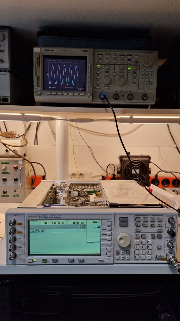
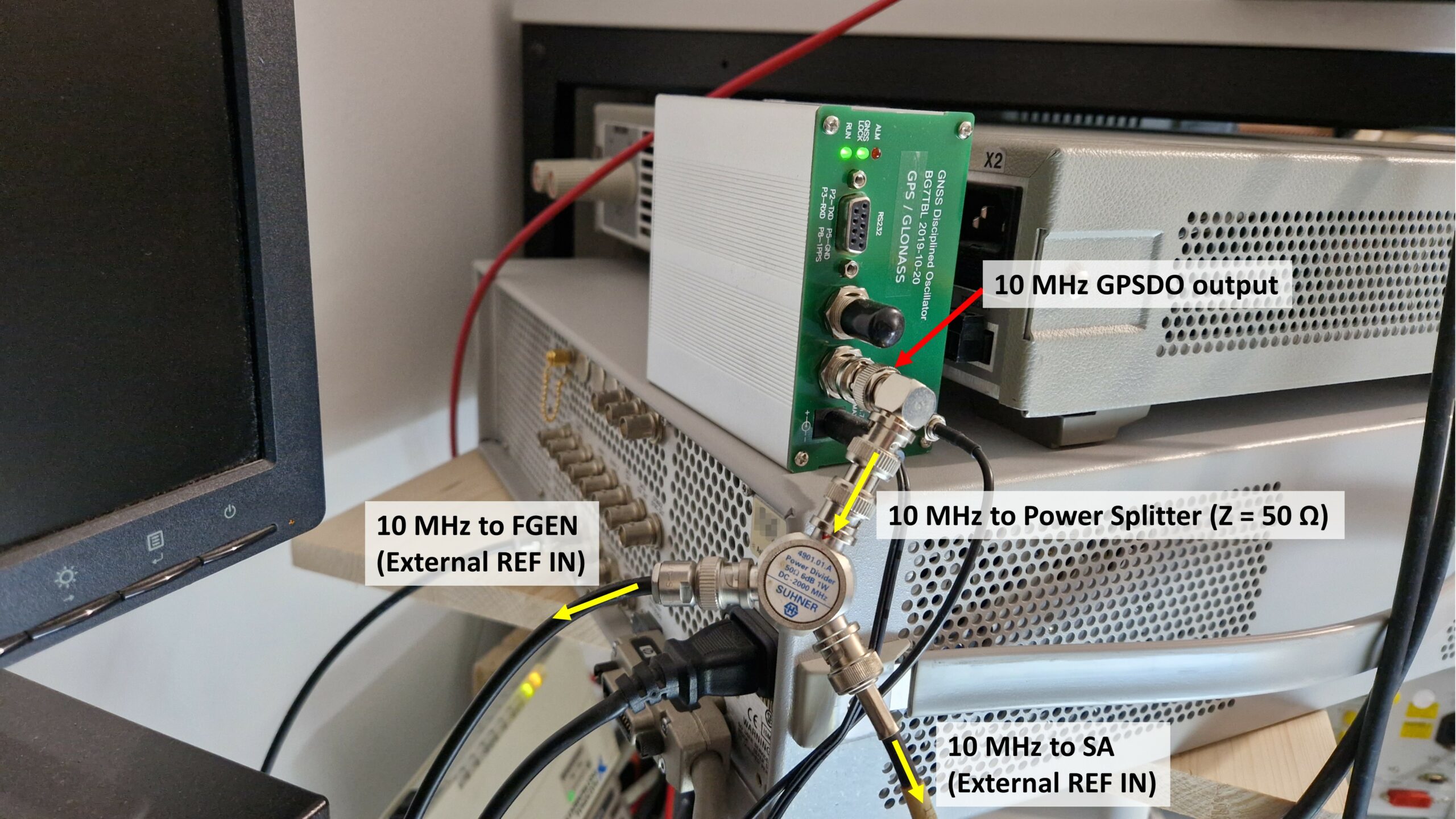
Long story short: I wasn’t disappointed and the SA works perfectly fine. I don’t want to write a lengthily blog about it. One of the first experiments was connecting my GPS disciplined oscillator to the signal generator and spectrum analyzer simultaneously in order to provide the same external reference for both instruments and checking if the frequency (1.5 GHz) and the amplitude (-35 dBm) are accurate. Acquiring measurements was super easy and the operation of the SA is very straight-forward.

Documentation of Measurements
I would consider the somewhat cumbersome recording of readings as a minor disadvantage of this SA. Taking a photograph of the display may be “quick and dirty” but you have to deal with bad image quality due to reflections, visible RGB pixels and picture alignment. It is possible to take screenshots in bitmap format (BMP) but one needs a special type of a Memory Card (basically a PCMCIA or PC Card) in order to save the screenshots on an external storage. That’s really unfortunate but measuring instruments of that era were either equipped by a floppy disk or Memory Carc. I was always afraid of damaging the fragile pins while pushing the PCMCIA card in its slot although it is rated for 10k mating cycles. The MS2661N type SA even has a 75 Ohm composite out – it’s possible to record video stills in the NTSC format. However, there are two elegant methods which I would like to show how to transfer the readout from the instrument to the personal computer (PC) by modern means.

Method 1: Sending a Hard Copy from SA to a PC
Back in the days, the measurement results such as frequency spectra would be printed on a piece of paper as a part of the documentation. A device called printer or plotter was needed and the process was called “hard copy”. The difference between a printer and plotter is how the drawing is generated: while the printer generates text and images line by line, a plotter can draw vectors in a X-Y-coordinate system. HP developed its own printer control language back in 1977 for this purpose – the HP-GL or Hewlett-Packard Graphics Language. HP-GL consists of a set of commands like PU (pen up), PD (pen down), PAxx,yy (plot absoute) and PRxx,yy (plot relative) in order to control a plotter, which is basically an electro-mechanically actuated pen. The commands are transmitted in plain ASCII via GPIB or RS-232C interfaces. If we were somehow able to capture the HP-GL ASCII code, it should be possible to generate a lossless vector graphics instead of a lossy bitmap.

Hardware Requirements
Besides the already mentioned spectrum analyzer one needs either a GPIB/USB or GPIB/Ethernet adapter. I have tested it successfully with a National Instruments GPIB-ENET/100 on a Windows 10 machine with NI 488.2 v17.6 drivers. It should also work with a NI GPIB-USB-HS+ (Chinese clone) adapter.
Software Requirements
I was looking for a quick solution how to acquire hard copies. Thanks to einball on a certain Discord channel 😉 for showing me the KE5FX 7470.EXE HP-GL/2 Plotter Emulator. John Miles, KE5FX, already wrote a software back in 2001 which does emulate a HP 7470A pen plotter. The 7470.EXE is still maintained by John and supports popular spectrum analyzers from HP and Tektronix. His software is able to fetch the HP-GL ASCII via GPIB and render the hard copy image on the screen. The image may be saved in a bitmap format (BMP, TIFF, GIF) or in a vector format (PLT, HGL). I have tested John’s software with Anritsu MS2661N and it worked perfectly fine. I suppose this could work on similar Anritsu spectrum analyzer models, such as MS2661C.
Setting up the Spectrum Analyzer
Here is a brief summary how to obtain a hard copy from an Anritsu MS2661N spectrum analyzer:
- Connect the spectrum analyzer to the GPIB adapter and boot up the device
- Go to the
Interface menuand use settings as followed → GPIB My Address:1, Connect to Controller:NONE, Connect to Prt/Plt:GPIB, Connect to Peripheral:NONE
The SA wants to send its data via GPIB to a plotter. It’s important to disable the “Connect to Controller” option, otherwise it won’t be possible to select GPIB as “Connect to Prt/Plt”. The GPIB address is set arbitrarily to 1 - Go to
Copy Contmenu (Page 1) → SelectPlotter Copy Contmenu (Page 2) → Plotter Setup → Select following options:HP-GL, Paper Size:A4 Full Size, Location:Auto, Item:All, Plotter Address:2
It’s important to set the “Plotter Address” value to a different number than the “GPIB My Address“. If both addresses share the same number, the hard copy will result in a timeout error
Install John’s 7470.EXE software and start the HP 7470A Emulator. There is no need to change the settings of the GPIB controller, it works out of the box. Click on GPIB → Plotter addressable at 2. The selected address in 7470.EXE should be identical as the previously set Plotter Address. In order to obtain a hard copy, press the button w and the 7470.EXE should display a message like shown in the screenshot below. Once you press the Copy button on the spectrum analyzer, a data transfer progress should be visible. It takes about 10-15 seconds to transfer the data (approx 7-10 kb) from the SA to the PC. Once it’s complete, an image of the current frequency spectrum is shown on the display. That’s it.


Creating Publication-Quality Vector Images
At this point, it’s possible to save the acquired hard copy in a bitmap image format. If one needs a publication quality images – which should be free of compression artifacts – one should save the images in a vector format such as PLT/HPGL. This workflow proved to be a little bit inconvenient but it’s perfectly doable. Save the hard copy as .PLT and open the image in a HP-GL supported viewer. John suggests few of them on his website – I’ve tried CERN’s HP-GL viewer. It’s distributed free of charge and still maintained by the developers. Download their viewer and load the PLT-image. If the colors seem wrong, there is a setting where you can change the pen colors. Once done, it’s possible to export the PLT image as PostScript (PS) or Encapsulated PostScript (EPS) or print as PDF. EPS files can be embedded in LaTeX documents or can be imported in a vector graphics editor such as Inkscape.


The results turned out to be really good. Especially the vector images are crisp and sharp. One can zoom in without any image quality losses. The printouts on my laser printer are perfect. A little downside would be few breaks in the workflow: one has to use three different applications in order to obtain, convert and process the images. But it’s worth it 😉
Method 2: Readout Data via pyvisa and Plot it via Matplotlib
A different method to plot the frequency spectra would be by downloading the acquired raw data via GPIB and plot it directly. This is exactly what I’ve done. I’ll share the Python code down below. It’s possible to refine the plot by automating more stuff: one can generate annotations directly from queried instrument settings. Just put enough time in it and you’ll get superb results. The plotted image can be saved directly in a Scalable Vector Graphics (SVG) or any supported bitmap/compressed format.
# -*- coding: utf-8 -*-
"""
Created on Tue Jan 3 16:45:39 2023
@author: DH7DN
"""
import numpy as np
import pyvisa
import pandas as pd
import matplotlib.pyplot as plt
#%% Open the pyvisa Resource Manager
rm = pyvisa.ResourceManager()
print(rm.list_resources())
#%% Create the Spectrum Analyzer object for Anritsu MS2661N at GPIB address 13
sa = rm.open_resource('GPIB0::13::INSTR')
# Print the *IDN? query
print(sa.query('*IDN?'))
#%% Take a measurement
# Set frequency mode to CENTER-SPAN
sa.write('FRQ 0')
# Set the center frequency in Hz
cf = 1.5E9
sa.write('CF ' + str(cf) + ' HZ')
# Set span in Hz
span = 10000
sa.write('SP ' + str(span) + ' HZ')
# Take a frequency sweep (TS)
sa.write('TS')
# Select ASCII DATA with 'BIN 0' according to Programming Manual
print(sa.write('BIN 0'))
# Create a Python pandas Series
data = pd.Series([], dtype=object)
# Fetch data, convert string to float, print the power level values
for i in np.arange(501):
data[i] = float(sa.query('XMA? ' + str(i) + ',1')) * 0.01
print(data[i])
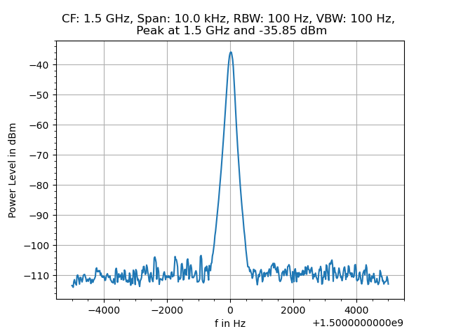
#%% Plot the results
# Generate the frequency values for the x-axis
f = np.linspace(cf-span/2, cf+span/2, 501)
# Plot the results, set a title and label the axes
plt.plot(f, data)
plt.xlabel('f in Hz')
plt.ylabel('Power Level in dBm')
plt.title('CF: 1.5 GHz, Span: 10.0 kHz, RBW: 100 Hz, VBW: 100 Hz, \n Peak at 1.5 GHz and -35.85 dBm')
plt.grid(axis='both')
plt.minorticks_on()
plt.show()
Few things to consider when using Python to obtain data from the spectrum analyzer:
- Anritsu MS2661N acquires only 501 data points per sweep
- The frequency axis values need to be generated manually. I used
numpy‘slinspacemethod. It was a bit tricky because you one has to change the generation of frequency step values depending on whether parameters “Center Frequency & Span” or “Start/Stop Frequency” are used - Fetching the data takes quite some time (approx. 30 seconds). This is due to the fact that every single data point needs to be queried with the
XMA?command in a for-loop. This is at least how it’s done in an example from Anritsu’s Programming Manual. I haven’t figured out yet how to fetch a block of data
Summary and Conclusion
I was clearly impressed how easy it was to obtain good quality frequency spectra images from a 20 year old instrument. I’ll refine the workflows and do further testing in Python. It should be possible to do all of this “automagically” via one little Python script. So far I’m really happy with the results where I don’t have to rely on smartphone pictures anymore. Thanks to einball for his help (basically googling for me) and to John (KE5FX) for writing his plotter emulator which helped me a lot to obtain hard copies from my SA. That’s it for today! Happy measurements! 😉
73 de Denis, DH7DN
Anritsu MS2661N Spectrum Analyzer Readout Read More »