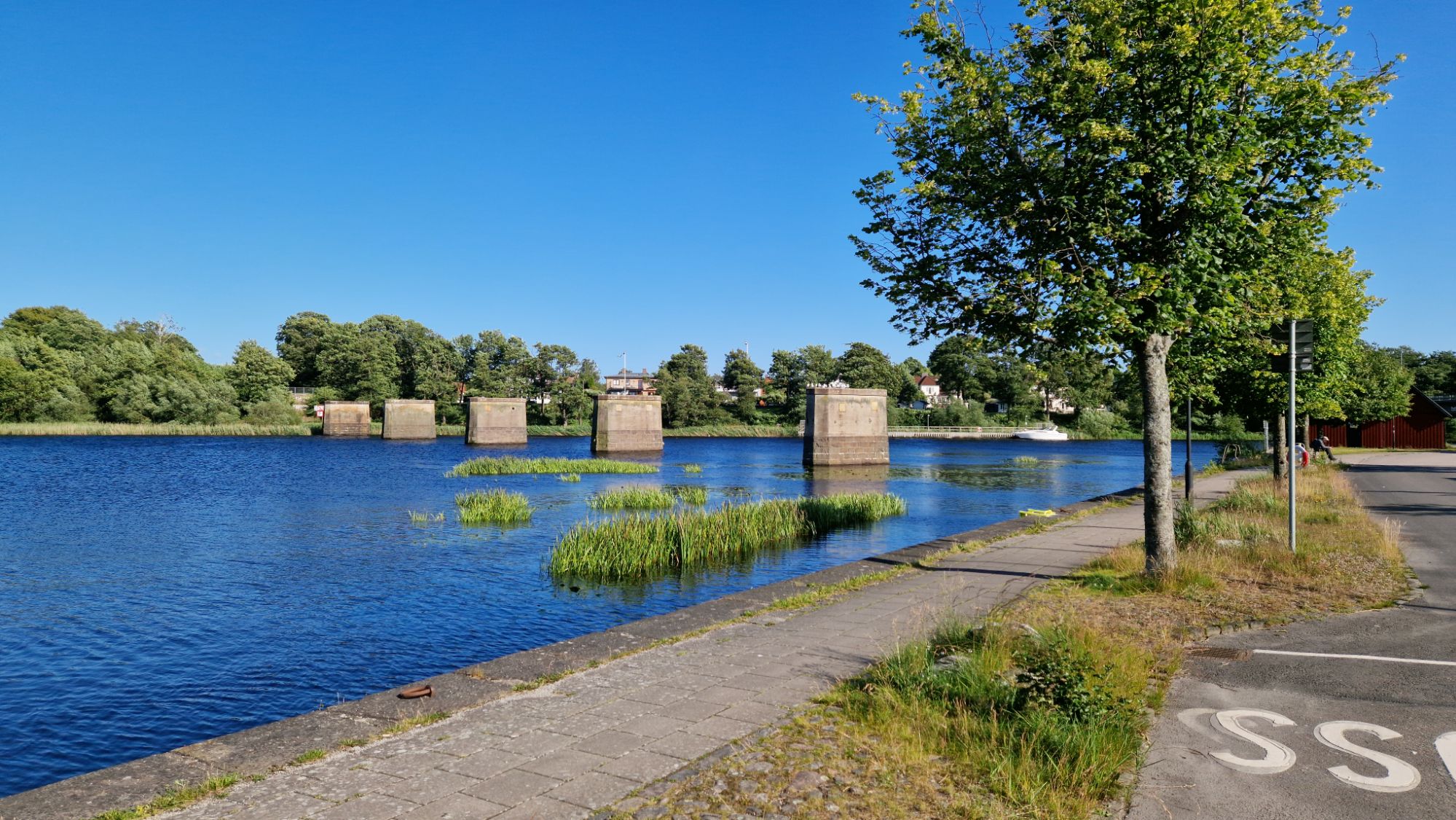
It’s already Monday! 😅 I had a great night at the camping site. It was calm and no noise from pesky humans. After check-out at 9:30am, I headed north-east along the western coastline of Vänern.
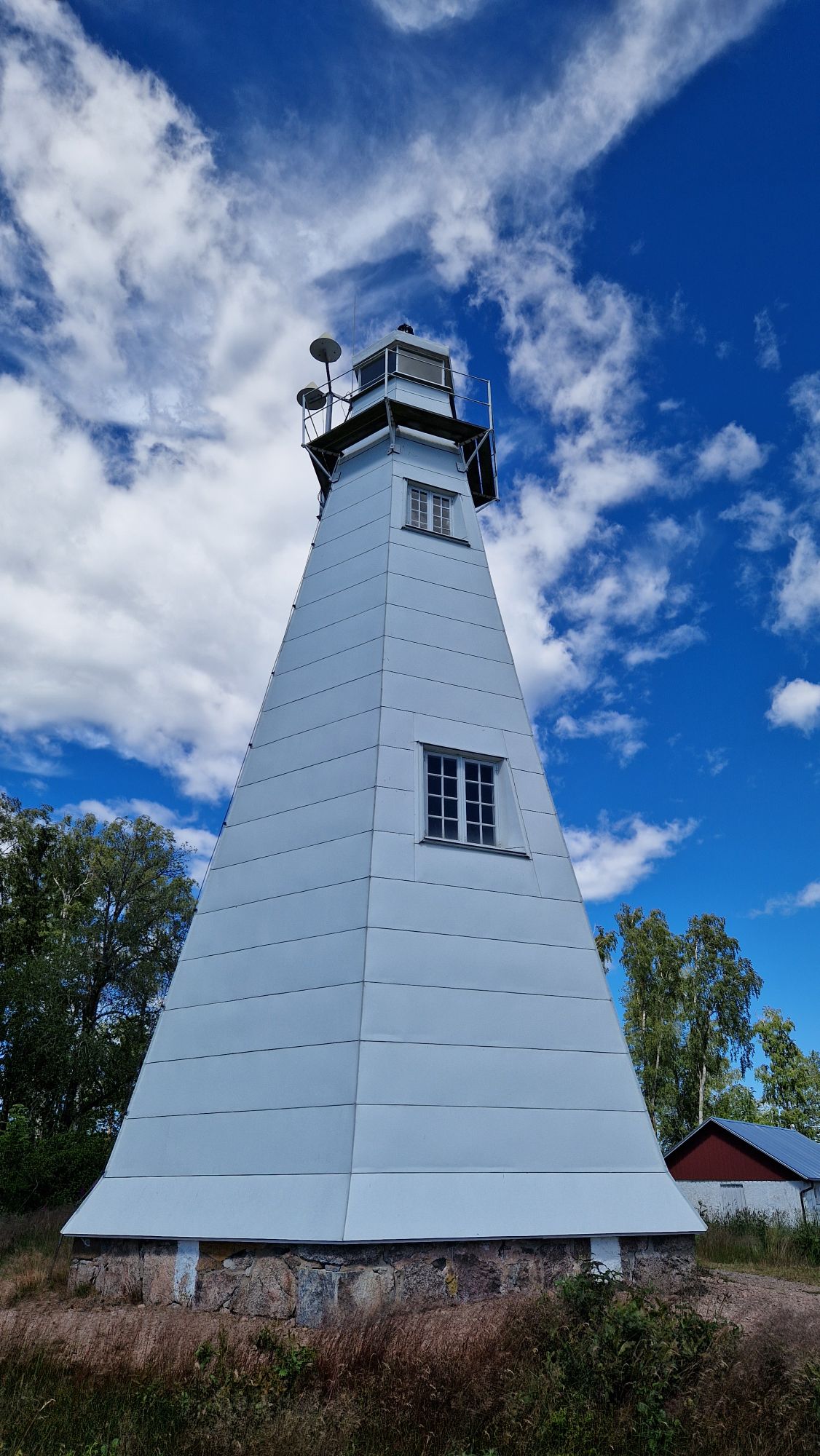
The weather was very nice for cycling: sunshine with little wind and no clouds with temperatures ranging from 19…25 °C. I’ve visited the lighthouse close to Jakobsbyn and it was really beautiful there. The cycle route No. 6 continued towards Mellerud, a small nearby town.
The lightshouse near JakobsbynOne last view before leaving Vänern
I had to take a longer break in Mellerud because I got tired really bad. Coffee and chocolate bars from a local gas station revived me again for the 2nd half of the tour towards Bengtsfors.
I cycled few kilometers with a cyclist from France, but the conversation was a bit difficult because of the surrounding noises (cars, wind) and language-specific accent. We parted our ways some 30ish km before Bengtsfors.
The route to Bengtsfors was simply beautiful. Lake on one side, forest on the other side of the road. Hills were steep and there were first signs of challenging terrain. The regional communities put a lot of effort to make this tourist region attractive…
Cycking along Lelång Lake
Anyways, I’ve been able to pursue my daily goals and reached a local camping grounds in Bengtsfors at 8pm. It has a lot of space and it’s located directly at the lake Lelång.
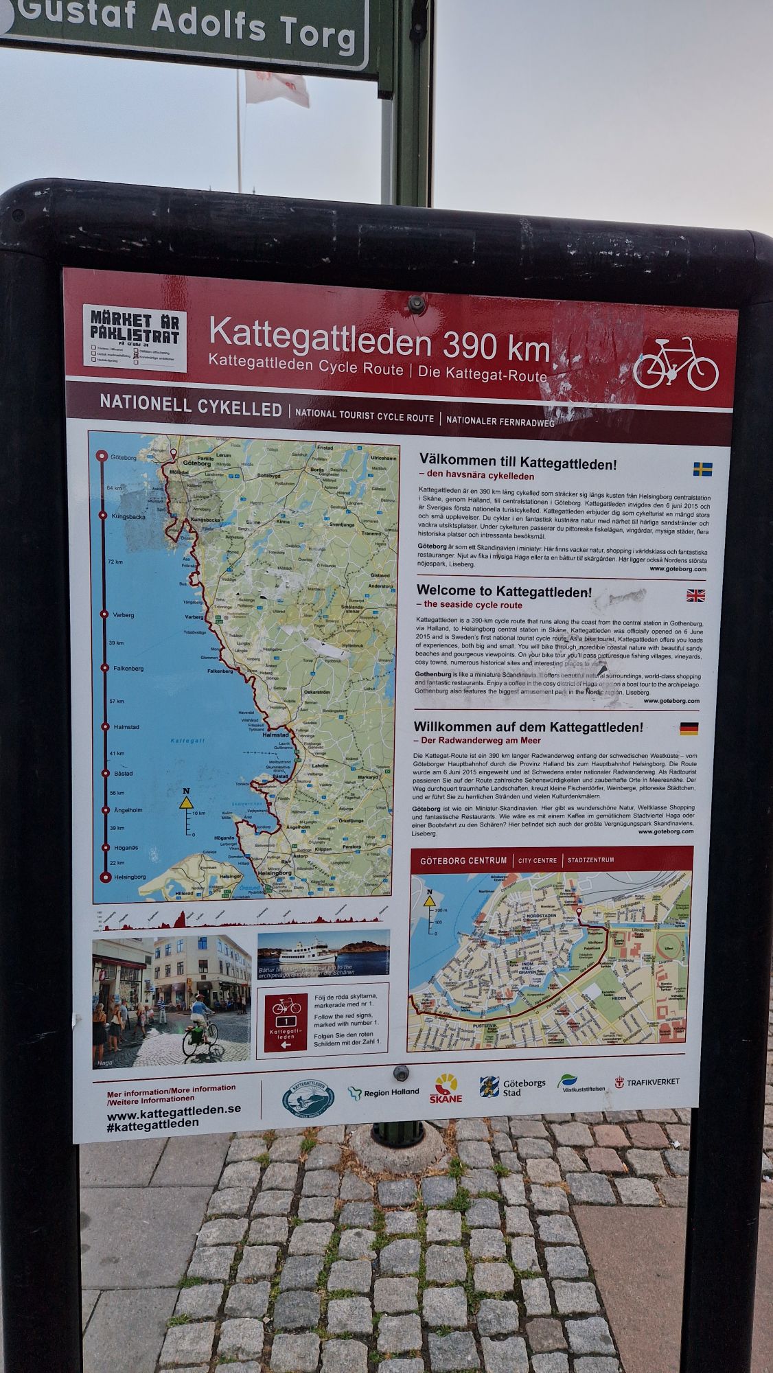
Sunday. My motivation got much better after eating up all the chocolate bars I had in storage. I cycled slowly some 10 km until I reached the Göteborg Central Station. I successfully finished the Kattengattleden from Malmö to Göteborg in 3 days, which was a huge motivator and also initial test (fitness, camping equipment).
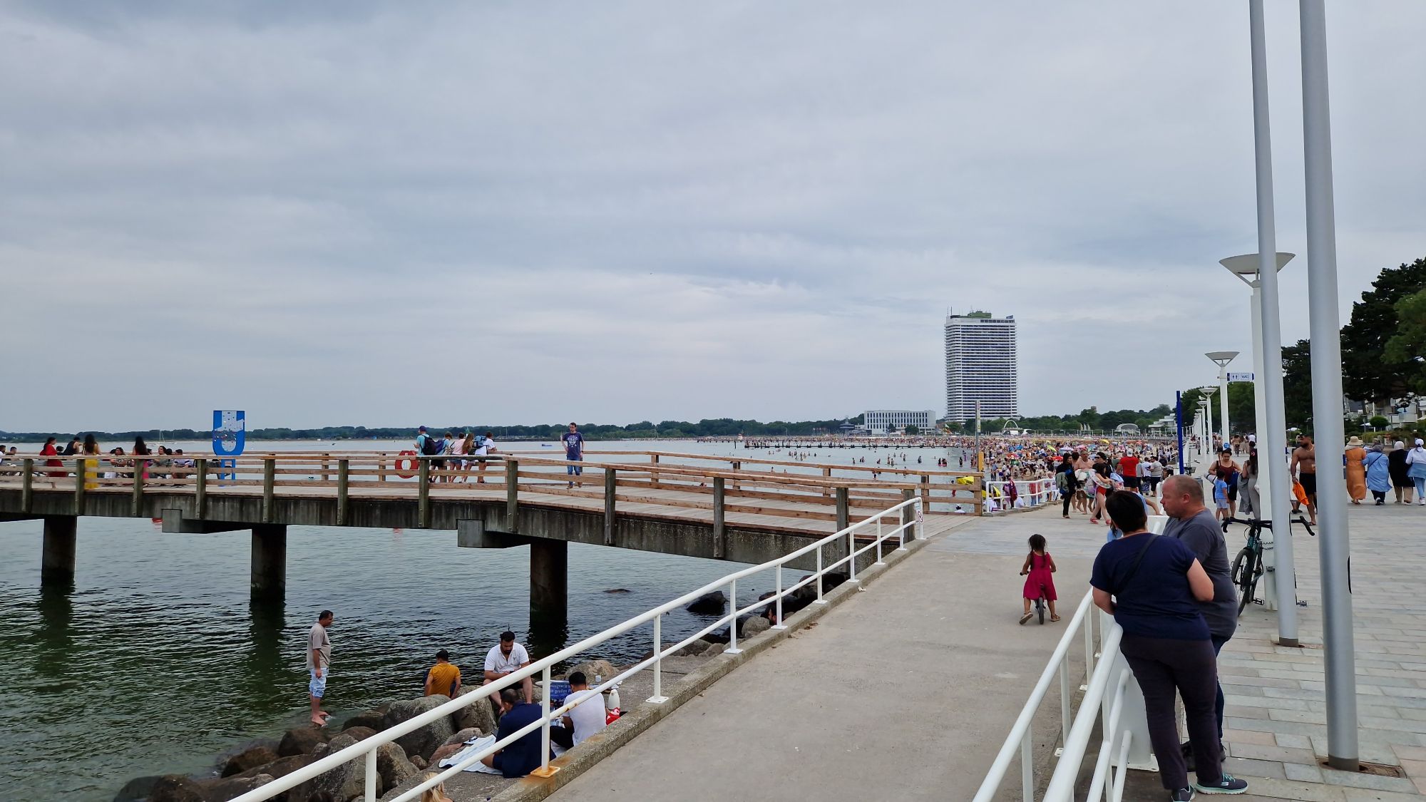
Göteborg harborVery impressive bridge in GöteborgKattegattleden completed! Success!
Unfortunately I realized that my planning had a flaw: there was no “Route 28” as suggested by OpenCycleMap and my waypoints didn’t match the town names on the direction signs. What a bummer! The backup plan was to use my smartphone to navigate – which increased the battery consumption significantly.
Nevertheless, I left Göteborg quickly and moved on. There wasn’t much to see on a Sunday morning around 5am (except the drunk party folks). Göteborg rather looked like a huge construction site than a city 😅 The toilet at the central station was out of order and I went to the gas station instead.
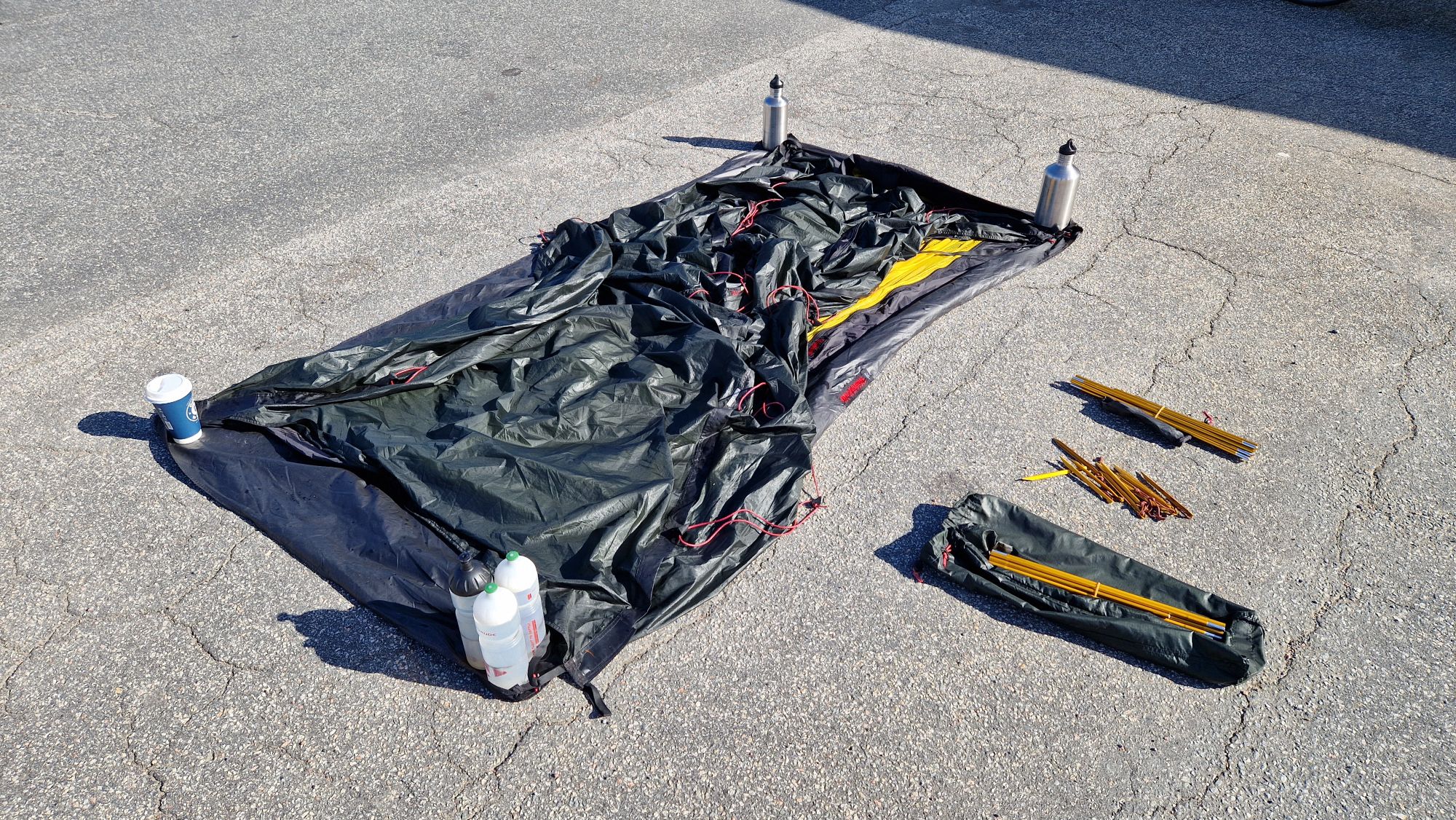
After a long phone call with mom, I stopped at a nearby gas station, bought a coffe and fuel and tried to dry my wet tent. There was enough sunshine and wind to blow it dry in like 20-30 minutes. This works great on asphalt since it absorbs some radiation from the sun and heats up the ground.
Drying my tent
I continued the bike ride at 11am and something amazing happened: for the next 70 km (!) or approx. 5 hours of riding time, I had a strong back wind which made the hills look like a piece of cake. I would have never thought this could happen. The back wind pushed my average speed up and I could reach Trollhättan and Venersborg between 4 pm and 6 pm respectively. The weather was perfect for cycling and the camping site at Vänern lake was amazing (except the price… 400 SEK or 35 EUR for one person with bike and tent). Unfortunatelly, the water was a bit too cold for my taste on this day 😅
This “TROLLYWOOD” imitation if the famous Hollywood sign in Trollhättan gave me a laughter!Vänern seen from the bridge……and from the camping site
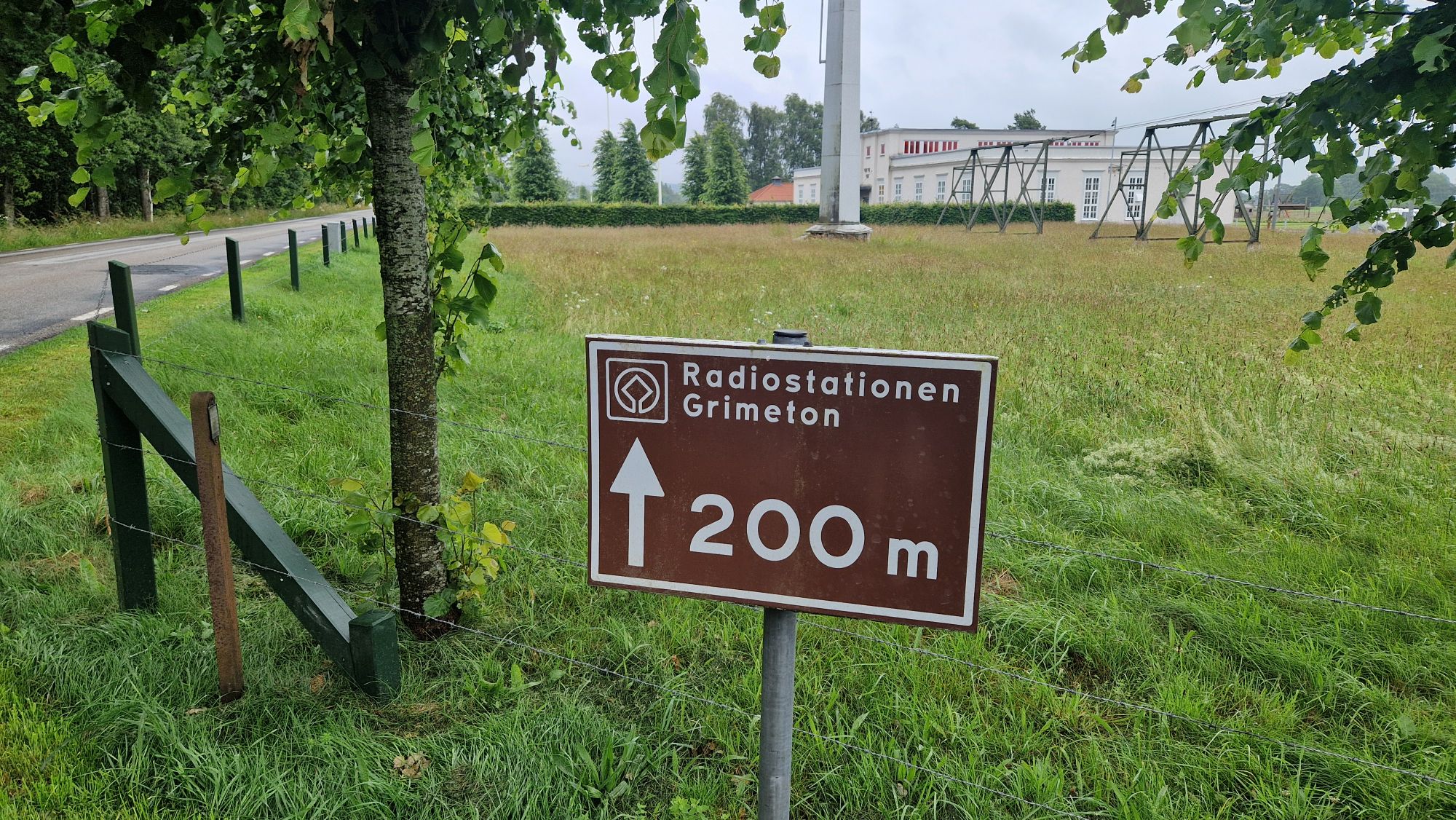
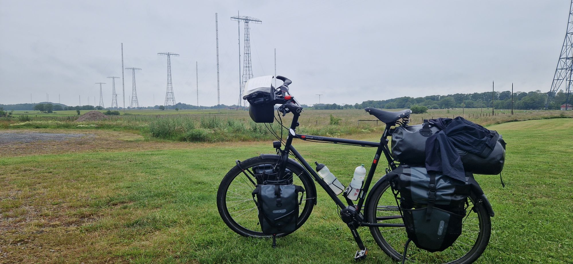
Saturday started with heavy wind and rain. I packed the wet tent and started cycling around 9:30am towards Varberg and ultimately to Grimeton. One of my goals of this journey was to visit the Grimeton Radio Station, the home of the Alexanderson Long Wave Transmitter – SAQ. Bad weather couldn’t stop me! I was there and saw the huge antennas, the transmission lines, the booth and some little extras. Unfortunatelly, I lost a lot of time for sightseeing and photographs but as always: #worthit. SAQ will transmit on July 2nd and celebrate its 100th birthday!
My short visit at the Grimeton Radio StationIn background: The huge antenna towers of the Alexanderson Transmitter in Grimeton
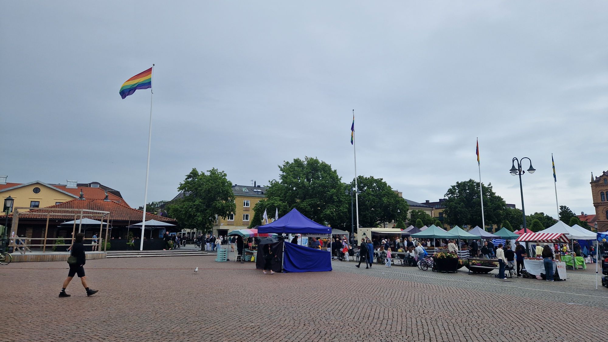
I continued the bike tour and visited the cities of Varberg (12 km) and Kungsbacka (50+ km after Varberg). In Kungsbacka, there was a huge Pride Parade and after randomly ordering a hamburger, I met a cyclist from Austria who was trying to cycle to Nordkapp! He had to cancel his travel to Nordkapp due to a bike defect with his spokes. We had a 20 minute chat about cycling, very nice guy.
Kungsbacka celebrating the Pride Day
Cycling to Göteborg took much more time than expected. Even with shortcuts to save some time and favoring weather conditions, I was still some 15 km away from the city and wasn’t able to find any camping grounds. The clock showed 22:30 hours and I had troubles reaching the daily goal. This of course ended in a bad situation for me… didn’t find a stay over night and camping inside or around Göteborg was virtually impossible. Had to sleep on a bench. Awful!
Noctilucent clouds over Göteborg
I did get maybe 2 hours of sleep, I was freezing, everything hurt after a long cycling day and it took a lot of effort to stay motivated.
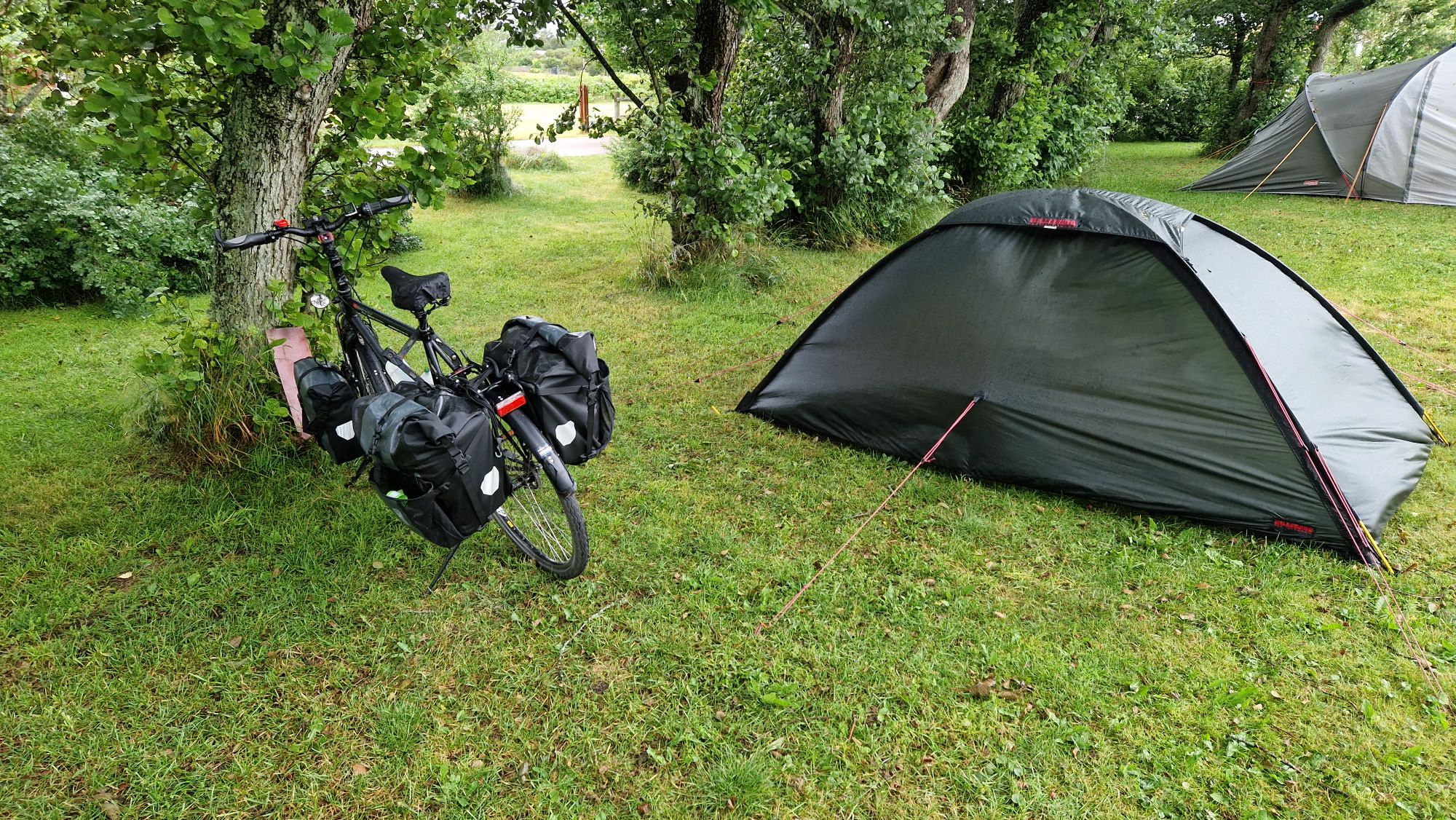
The previous night was rainy/windy. Luckily, as I woke up, the rain stopped and it was just windy. I packed my stuff and was en route a bit late at 9:30 am.
15 km till HalmstadSculpture in Halmstad
The rest of the day I was confronted with heavy headwinds. My average speed dropped from 16 km/h down to 13 km/h. Sounds not much but it’s significant. It usually means “double punishment”: cycle harder with less speed. I’ve visited Halmstad with quite some delay and cycled on towards Falkenberg. It was very exhausting but the weather got much better towards afternoon. The winds calmed down by evening hours around 6-7pm.
An unfinished “bridge” in Falkenberg
I couldn’t reach my daily goal Varberg, however, I camped in Björkäng, about 15 km away from Varberg. By luck, I met a wonderful traveller couple from Germany at the campsite in Björkäng who invited me for a coffee and travel-talk. They have been travelling in Sweden and Norway for the past 6 weeks by camping van and told me a lot about the special places they visited and I surely want to visit in the next couple of years. That was worth it… great experience!
A sun’s halo (rainbow patterns) spotted near Morup
Tomorrow I’ll continue my route to Varberg and head to Grimeton before finishing the Kattegatleden in Göteborg. Will try to keep 100 km/day as long as possible…
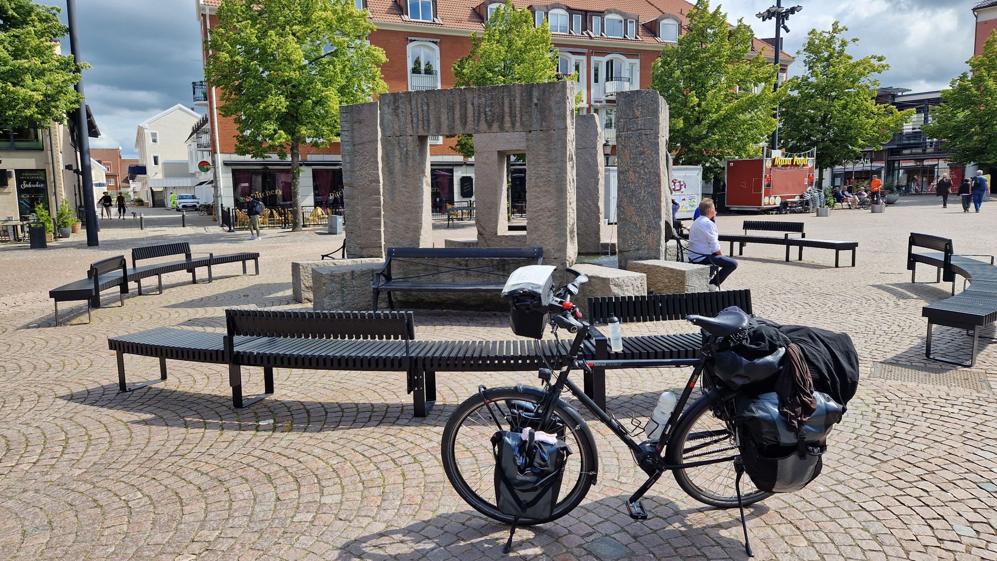
Very nice cycling day. The weather was perfect for cycling. First 30 km were very easy to master, however I started slacking and lost some time with shopping and breaks. The landscapes were beautiful and very pleasing.
Ängelholm center
My daily goal was to reach Halmstad, however, the weather report showed some incoming rain. I decided to camp in Laxvik just before the rain set in. That seemed to be the right decision because shortly after setting up the tent, it started raining.
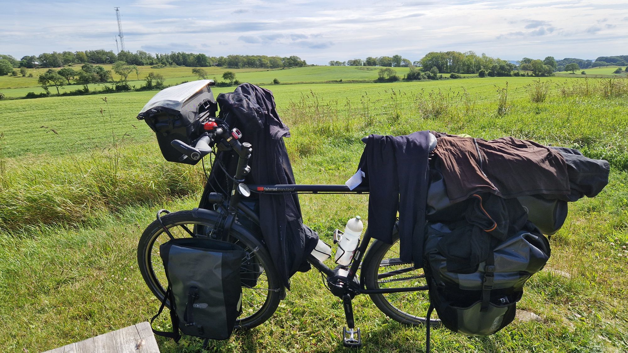
Taking a break and drying wet clothes
There was lot of rain with changing duration and intensity, followed by strong winds. I was very tired and just slept without caring much about the noise…
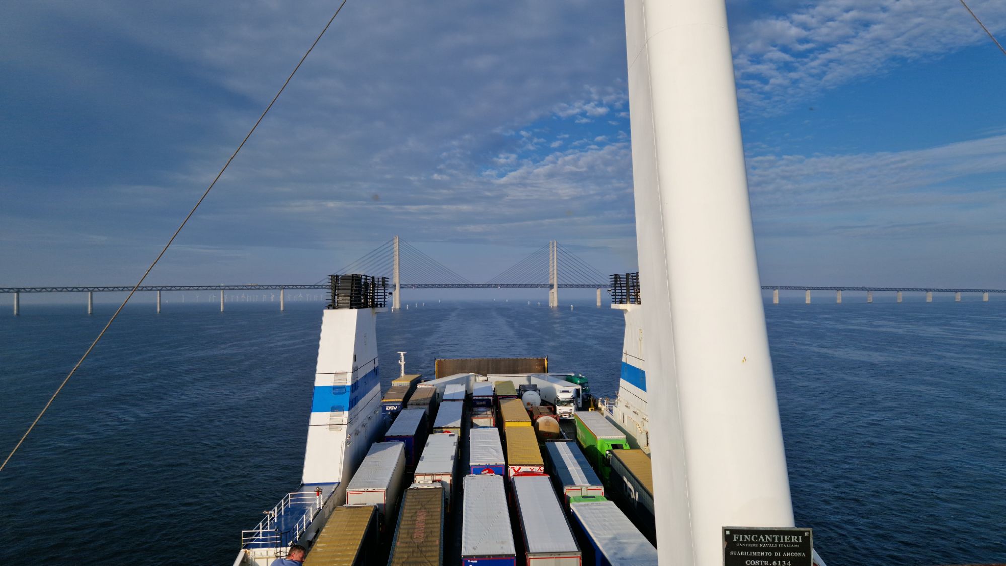
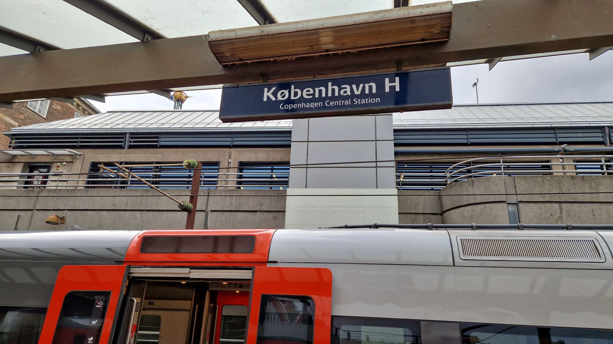
My bike tour started today on Wednesday, 2025-06-25. I woke up early in the morning at 5:30, packed my stuff and had some great breakfast. The Copenhagen Central Station was some 300 meters away. The ticket price from Copenhagen to Malmö was a bit cheaper (99 DKK for ticket and 50 DKK for bike ticket, ca. 20 EUR total) than the other way around.
Crossing the Øresund Bridge by train
The weather was mixed and windy at 18 °C. The first half of the day was windy and raining. Later during the afternoon, the weather got much better – lots of sunshine and no clouds. It was windy along the coastline, less windy towards main land.
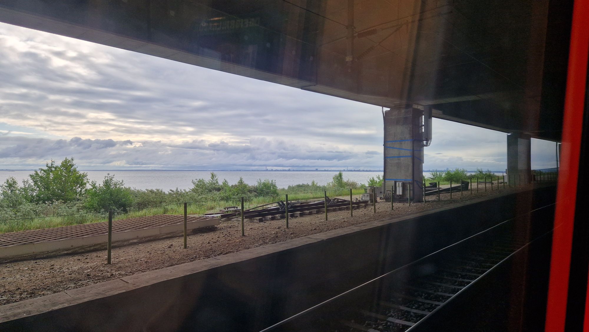
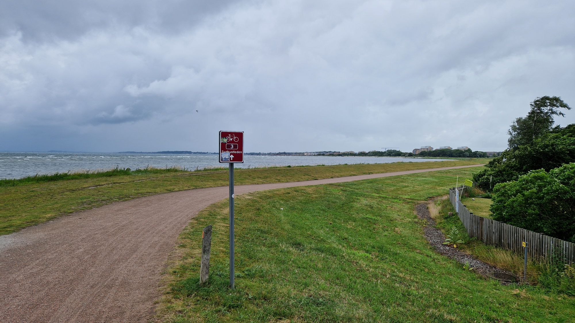
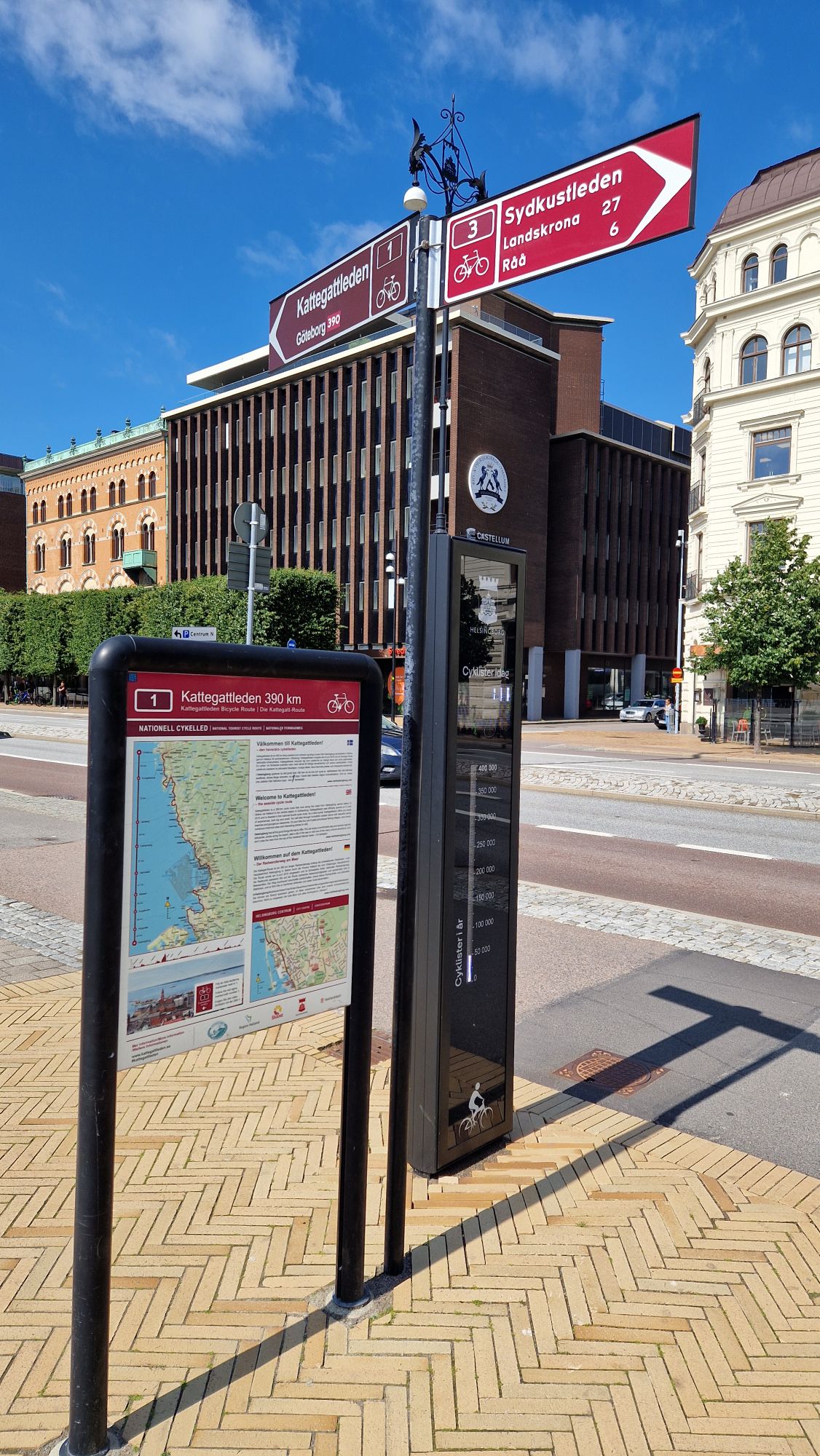
Sydkustleden – Cycle Route No. 3
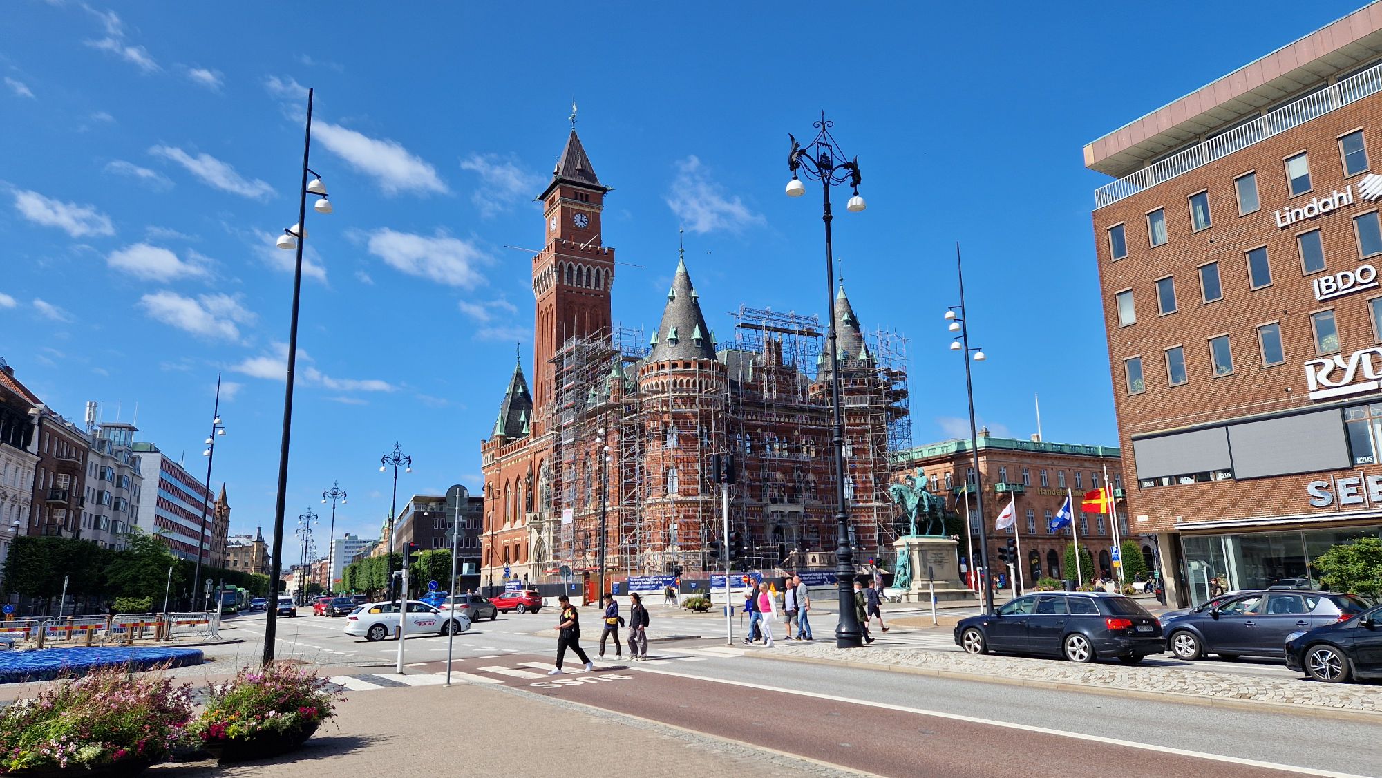
From Malmö C, I followed the route No. 3 – Sydkustleden to Helsingborg. I have visited cities of Landskrona and Helsingborg. In Helsingborg, the route was continued on Kattegatleden Cycle Route No. 1 to Göteborg.
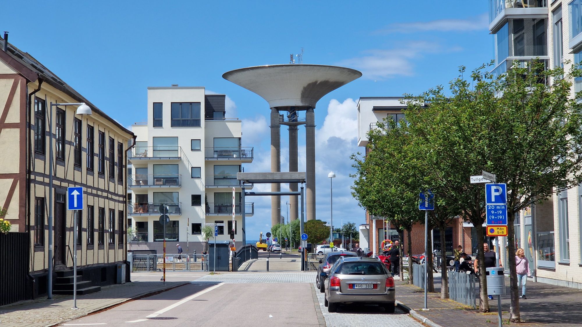
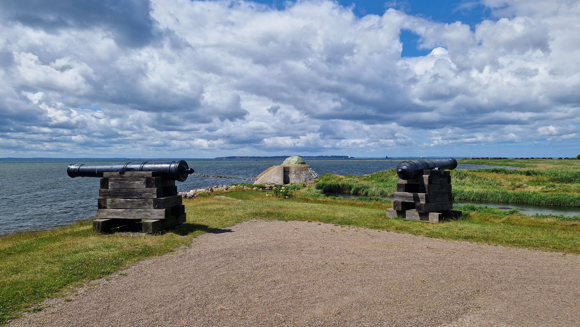
Flying saucer in LandskronaCannons and WW2 bunker near the Citadel in LandskronaHere we are in Helsingborg at the start of Kattegatleden Route No. 1 to GothenburgHelsingborg
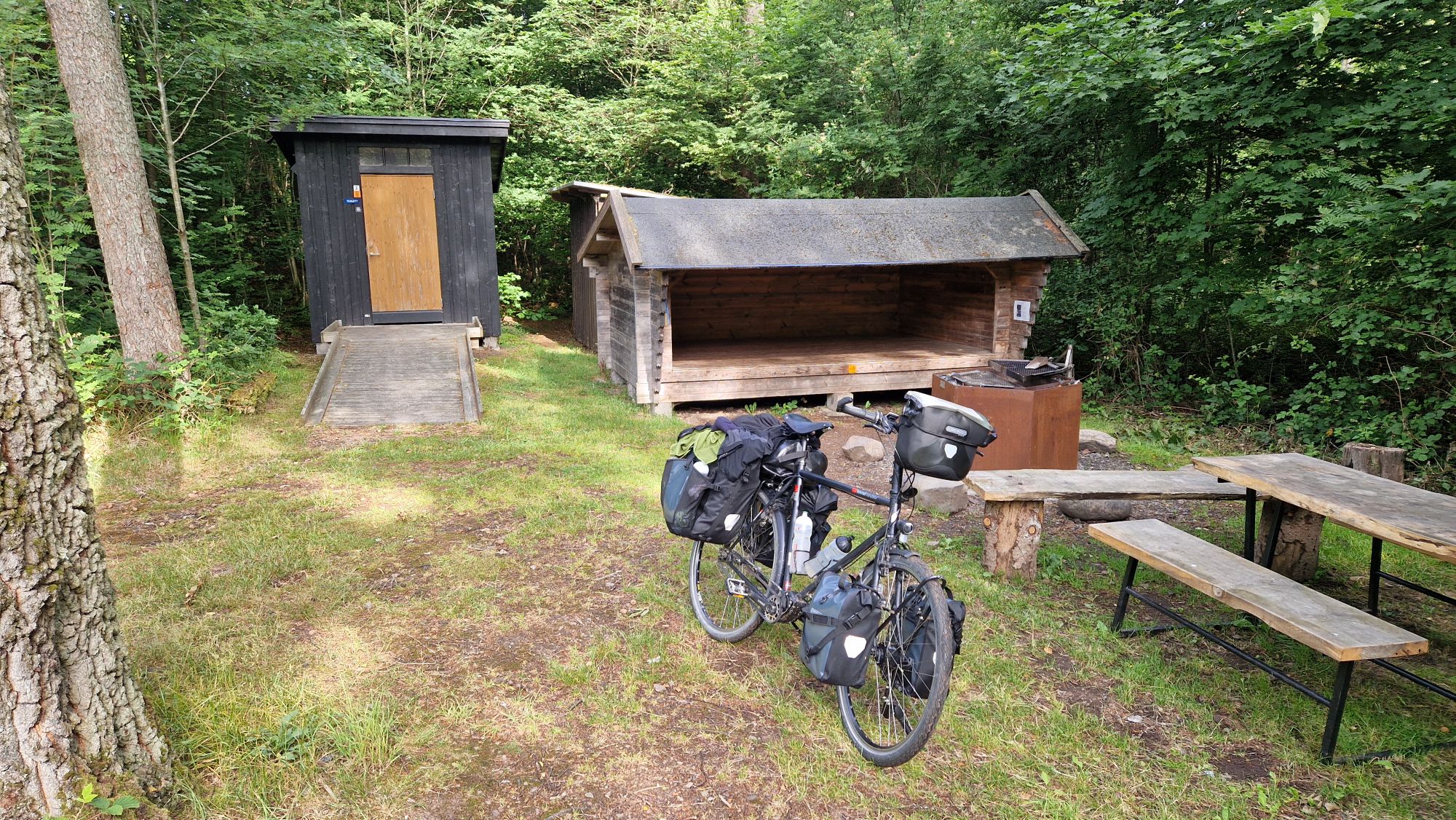
I kept cycling until late in the evening until tiredness set in and I had to find a place to rest. After looking for a camp spot, I found a shelter few kilometers behind Brunnby where I slept over night. Great place, it was quiet and I really enjoyed it.
Shelter near Brunnby
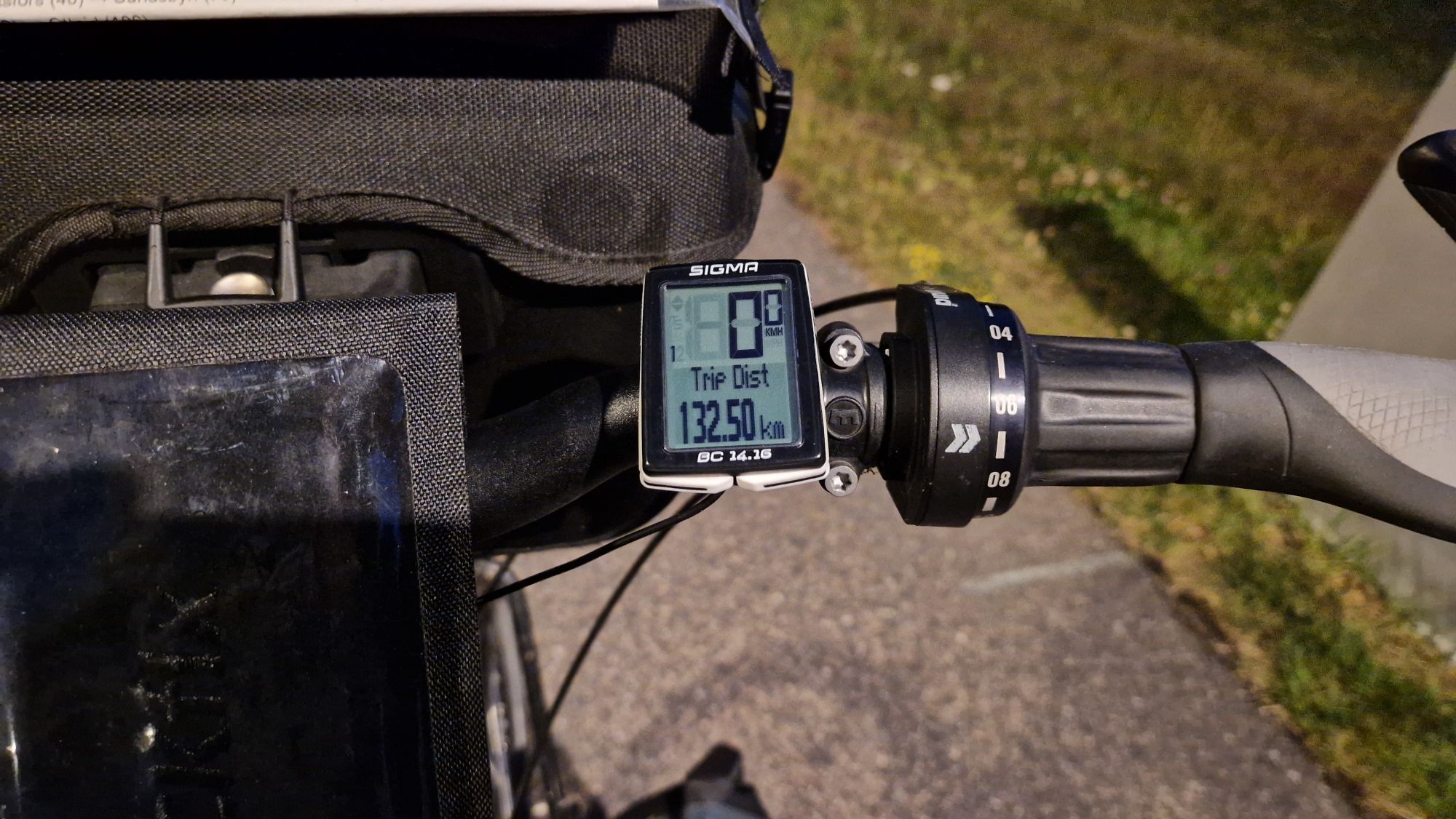
Total distance: 123.7 km, Ride time: 8h40m, average: 14.3 km/h
Staying today at Copenhagen to visit some places and to recharge batteries, resupply missing stuff etc.
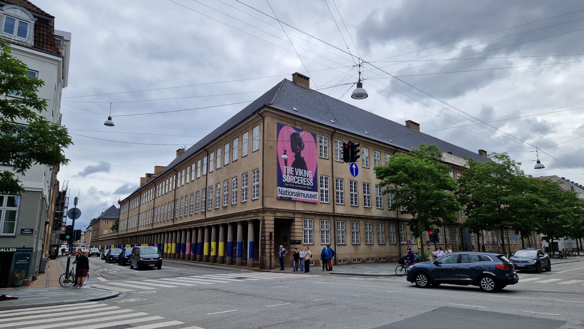
I visited the Danish National Museum and spent there few hours and participated in a guided tour. It was very interesting learning about Viking and Danish culture, ranging from the 10th century till modern times. I liked the museum very much, well spent money.
The Danish National Museum
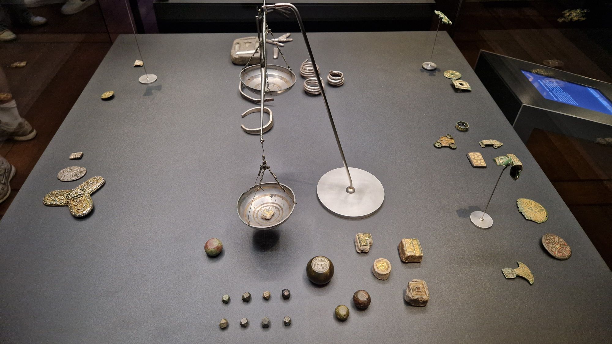
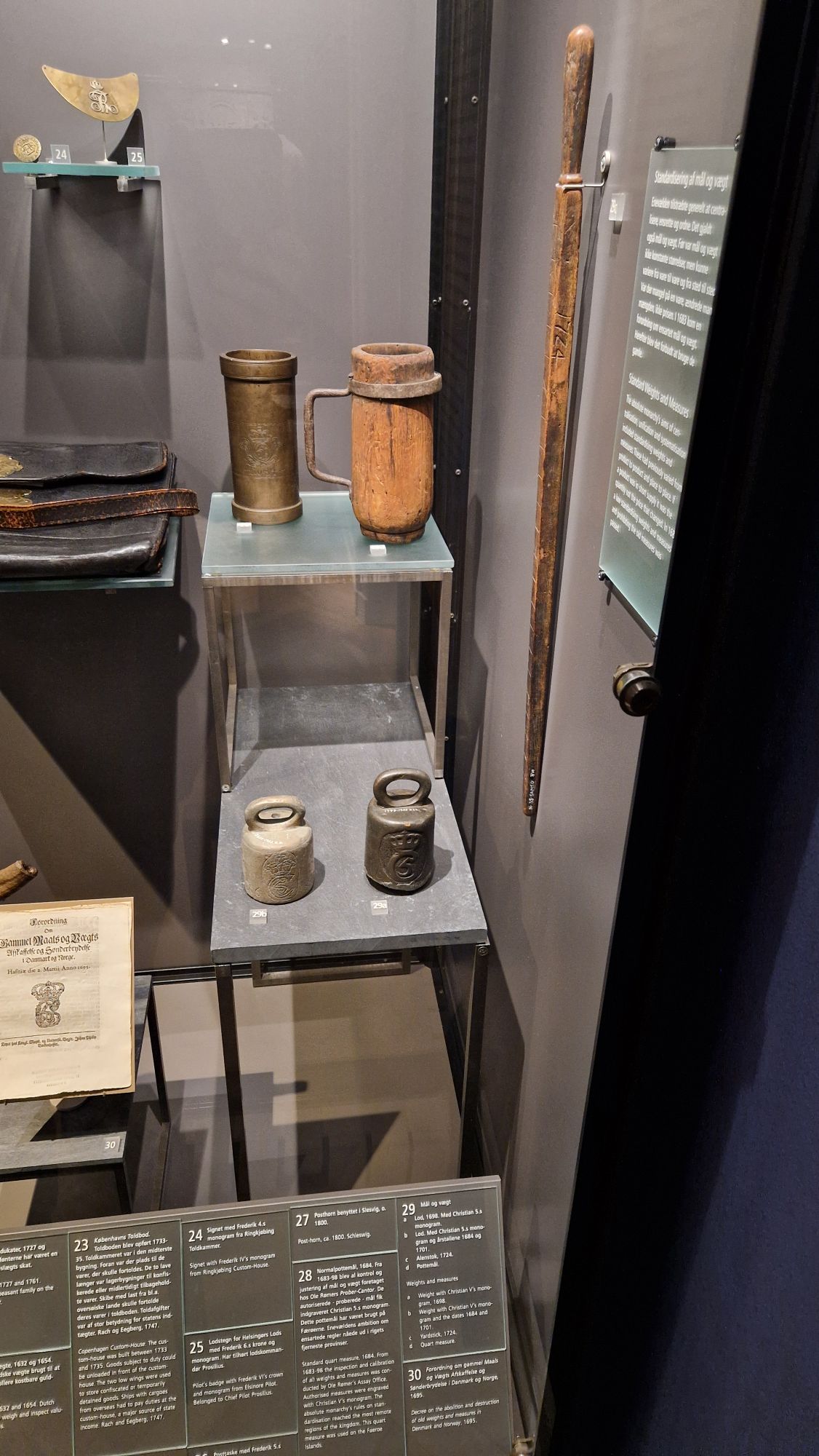
It’s funny how Vikings and – much later – the King of Denmark were “victims” 😅 of Metrology when it comes down to trade and economy. Typical trade goods back in those days were precious metals such as gold and silver or expensive spices (pepper, salt etc.). I couldn’t resist making some pictures of scales and their “weight standards”.
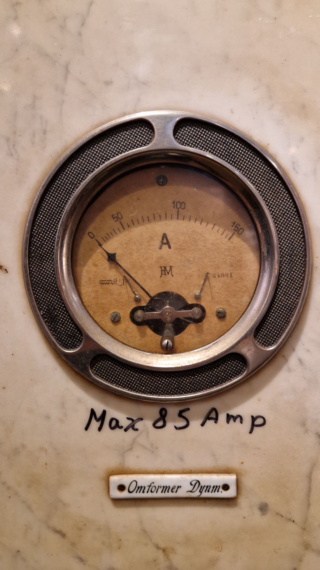
An ancient scales and some weight standards (small cubes/dices in front)Length, volume and weight “standards”Modern-day test equipment – an amperemeter from the early 20th century
After diving into history for 4.5 hours, I was finally looking for a fish restaurant but couldn’t find one which isn’t too expensive. I found one but prices for a menu were in the order of 40 EUR without drinks. Instead I decided to go to a grillhouse. The dish was very tasty but also pricy – almost 30 RUR for a grill menu. Usually it’s 20-ish EUR but eating in a shopping street proved to be very pricy.
BBQ at grillhouse
The weather didn’t recover much, temperatures were around 18 °C today with short periods of rain. I decided to return to the hostel and start preparations for the bike tour, which starts tomorrow. Unfortunatelly one of my roommates didn’t sound very healthy – he was coughing and stayed in the room presumeably the whole day. I hope he doesn’t give me a flu…
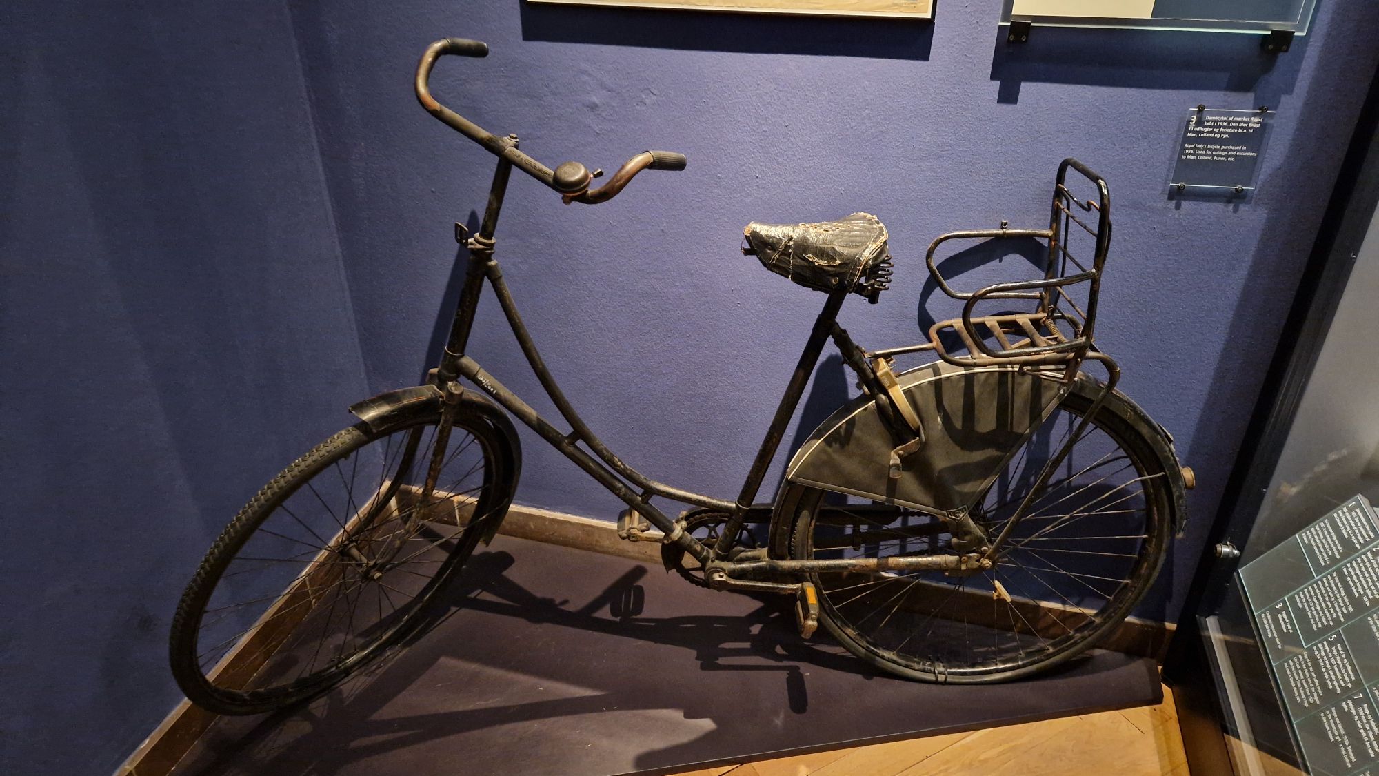
Not my bike, but it has much with the modern-day bikes in common…
Had a good night, slept very well. I missed the Øresund Bridge transit just by few minutes but was able to capture some awesome views shortly after the passage.
Just passed the Øresund Bridge
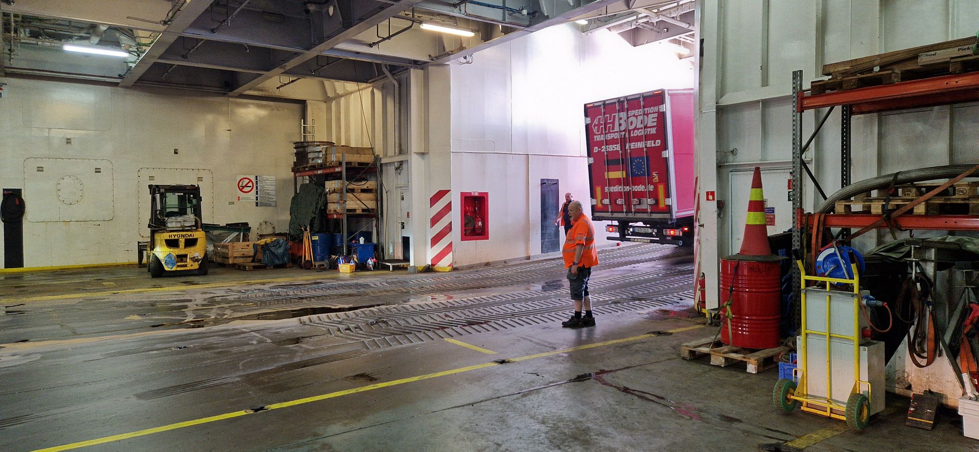
Breakfast was fine and going off-board went very smoothly – at least for me. Thanks again to the Finnlines crew!
Waiting for the sign to leave the ferry
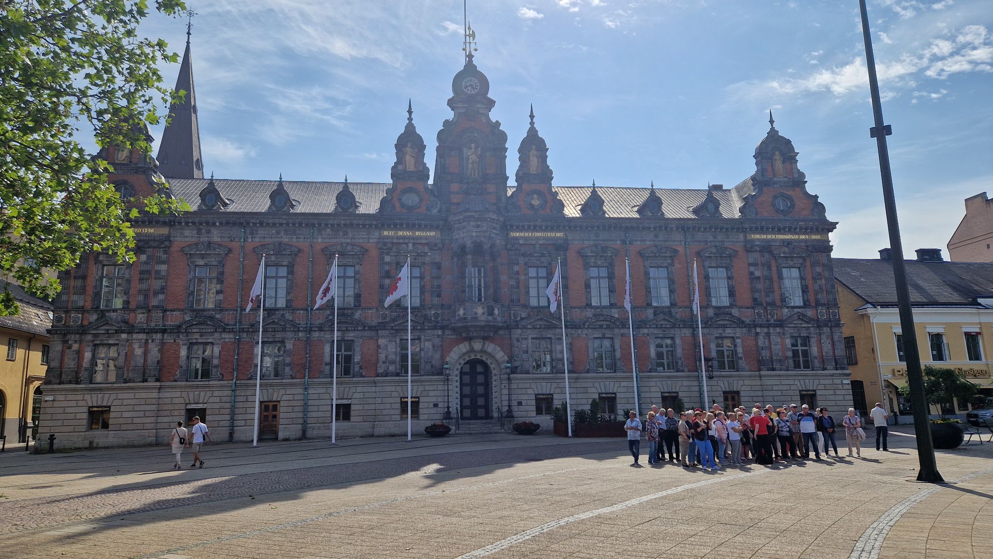
The weather was very good (20 °C) and I checked out the central station, the old town and the promenade of Malmö. After few hours of walking and weather change to wind/rain, I moved on to the Malmö central station and grabbed a train ticket towards Copenhagen. It cost me 220ish DKK which is around 30 EUR (bike ticket included).
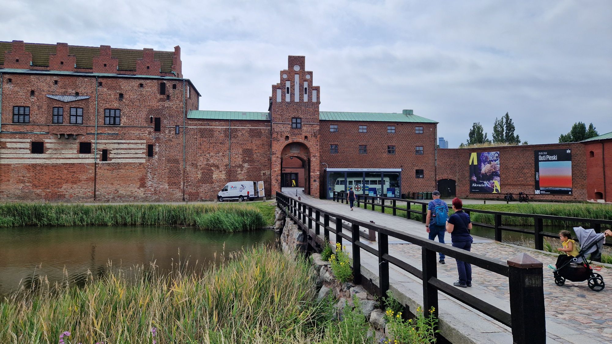
City Hall of MalmöKungsparken MalmöMalmöhus Museum
I arrived ~35 min later in Copenhagen. The view was spectacular when crossing the Øresund Bridge. Unfortunatelly, the train was full, couldn’t take any good photos. I checked in to my hostel where I will stay for the following two nights. The bike tour starts on Wednesday!
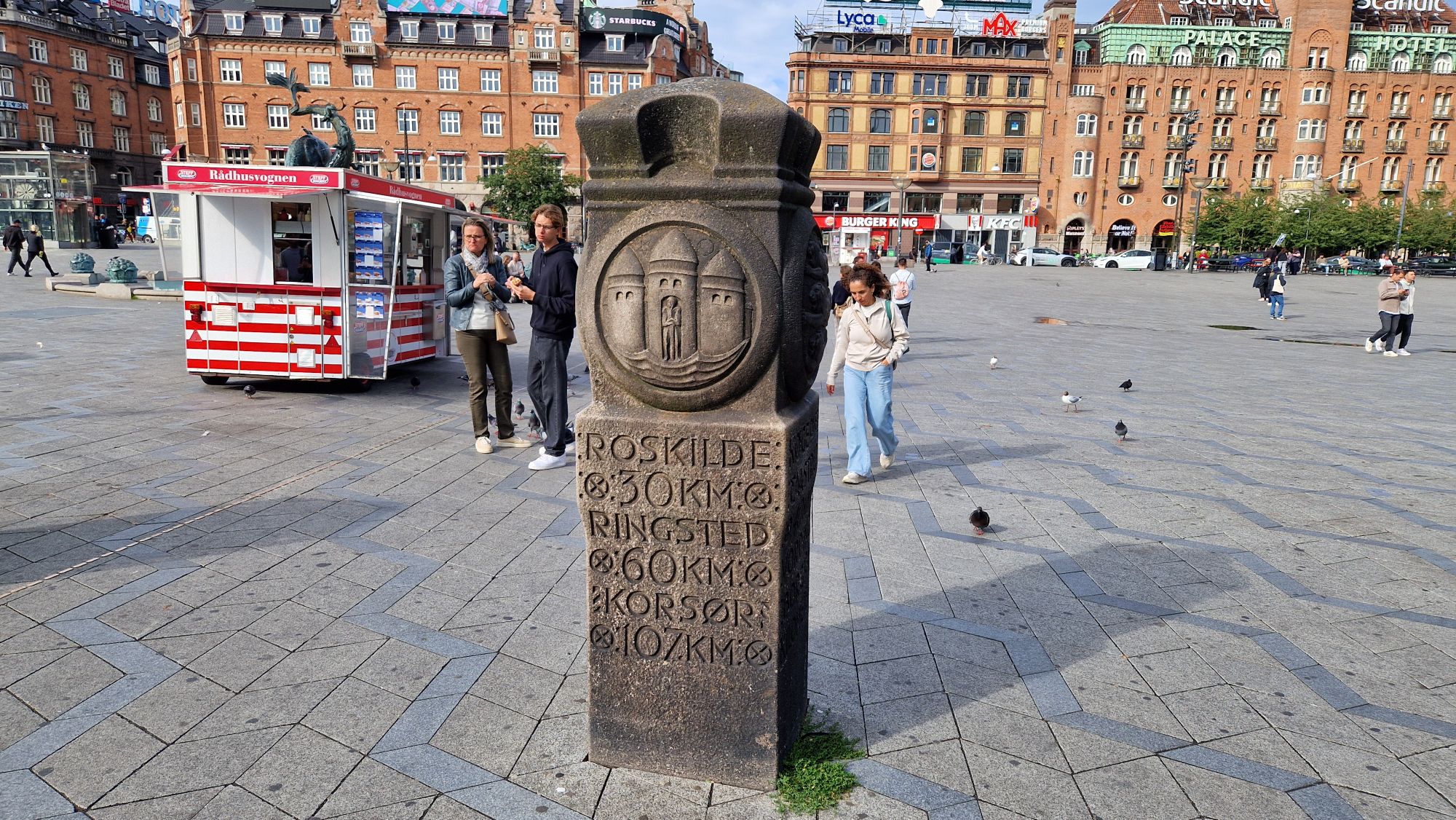
Arrival at Copenhagen Central StationMilestone in CopenhagenThe Danish Stock Exchange being rebuilt after its destruction by fire in 2024
This time I’m trying something new. I’m currently on vacation and I’m about on my way to ride my bike from Copenhagen, Denmark through Sweden to Bergen, Norway. I will try to write a travel blog on a daily basis via my smartphone through the next couple of weeks.
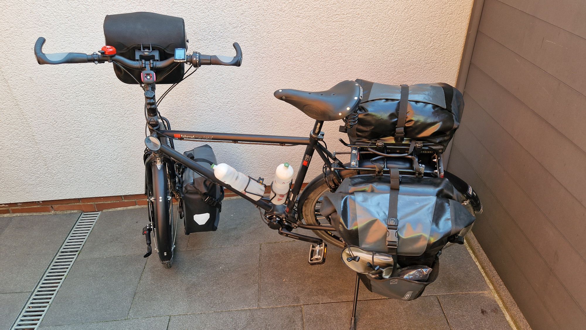
Basically, during past couple of days, I’ve been busy packing my stuff to travel via bike and tent. It took me three days to prepare everything (clean clothes and bike, repair equipment etc.). Packed the bags by sunday morning and hurried to the central train station.
vsf Fahrradmanufaktur TX-1200 packed
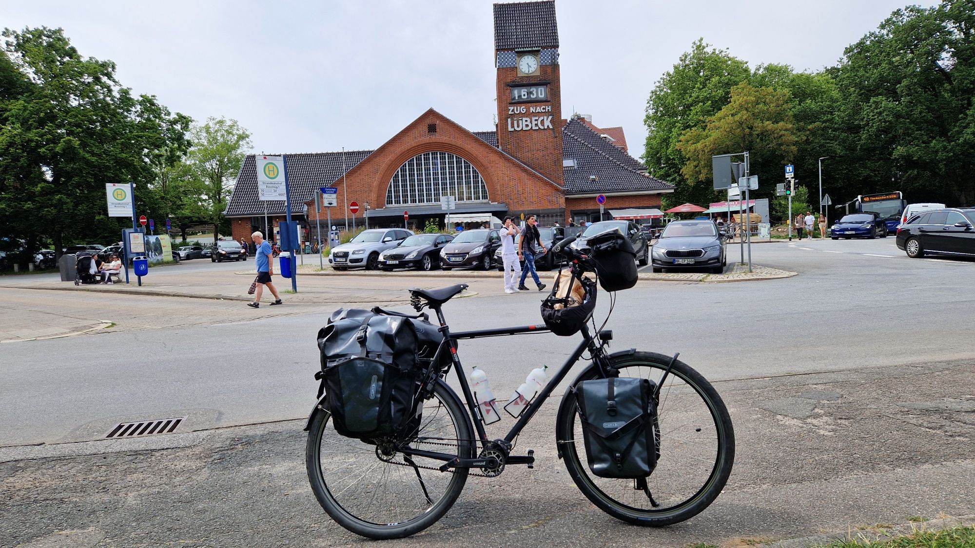
Catched the train on time and also arrived in Uelzen on time. However, the connection to Hamburg had a delay of approx. 40 min. Further delays forced me to change trains in Lüneburg in order to get to the city of Lübeck-Travemünde. I arrived about 1 hour late due to train delays but still had 3 hours left.
Arrival in Travemünde
I killed the time at the beach before moving to the harbor. The beach of Travemünde was crowded very well, temperature was around 27 °C.
Beach of Travemünde
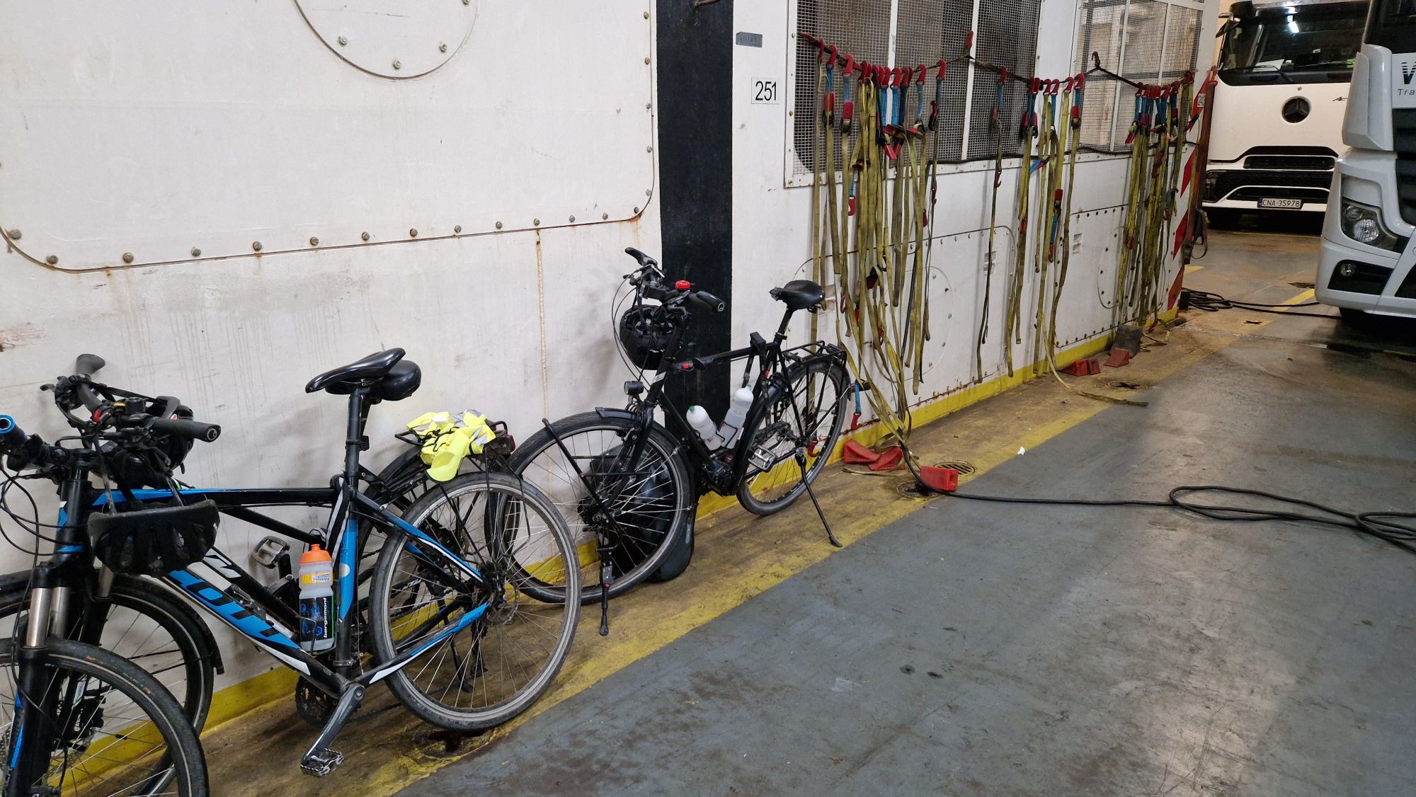
At around 18:30h I moved to the port towards Skandinavienkiel. The check-in at the port was very easy and I met some nice cyclists along the way. We went together on board and had an exclusive place for our bikes in front of the ship (bow side).
Our bikes at the car deck
Departure was on time at 22h and the sights from the Observation/Sun Deck were amazing – the promenade, the beach and some lightning on the horizon!
Leaving Travemünde
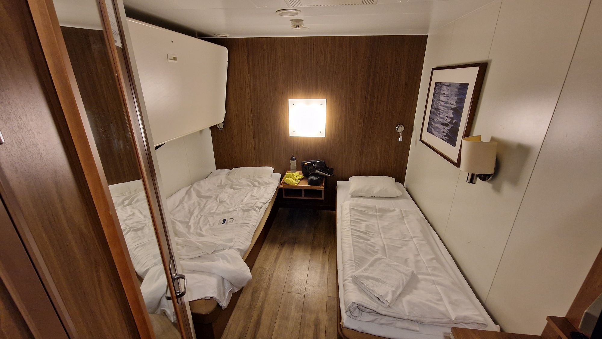
The Finnlines personnel were friendly and very supportive, thanks alot to the crew!After having a dinner, I went to the cabin and passed out quickly due to a dense packed travel day. Awesome!
I’m a bit out of phase (2 weeks late) but it’s cold and dark outside, maybe I’ll write some blog articles soon(tm) 😅
There will be interesting stuff in 2025, namely electrometers, voltage references, more cycling adventures, ham radio stuff and… screws! Lots of screws…
Just a fistful of screws. I wonder where they belong …
I have been very busy during the past 3 months. I’ve prepared some blog posts but had no time or motivation to finish and publish them. Usually my blog posts have several hundreds or thousands of words with images which can be very time consuming when compared to microblogging services such as Twitter/X or Instagram and Mastodon. I’ll try to keep it brief this time 🙂
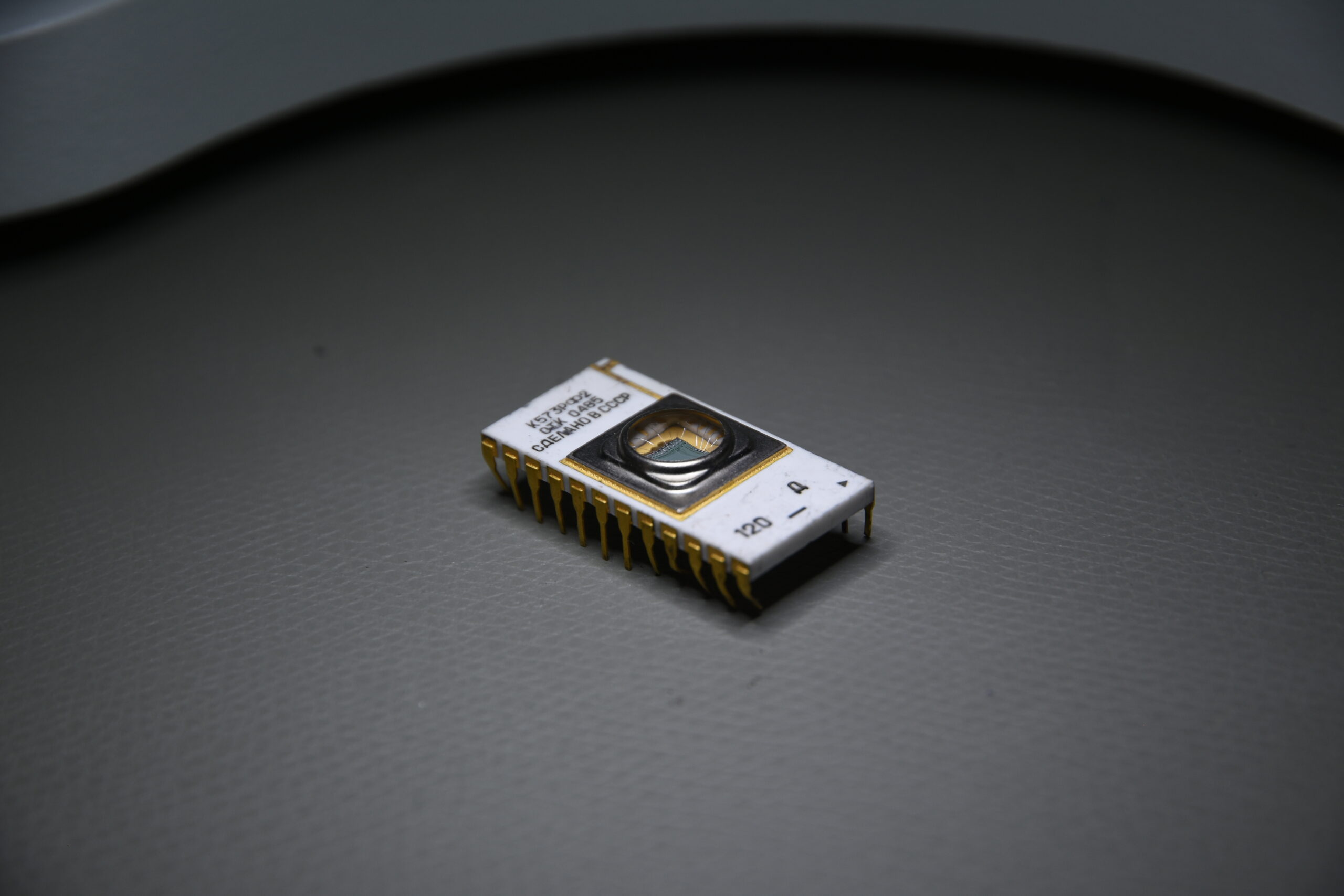
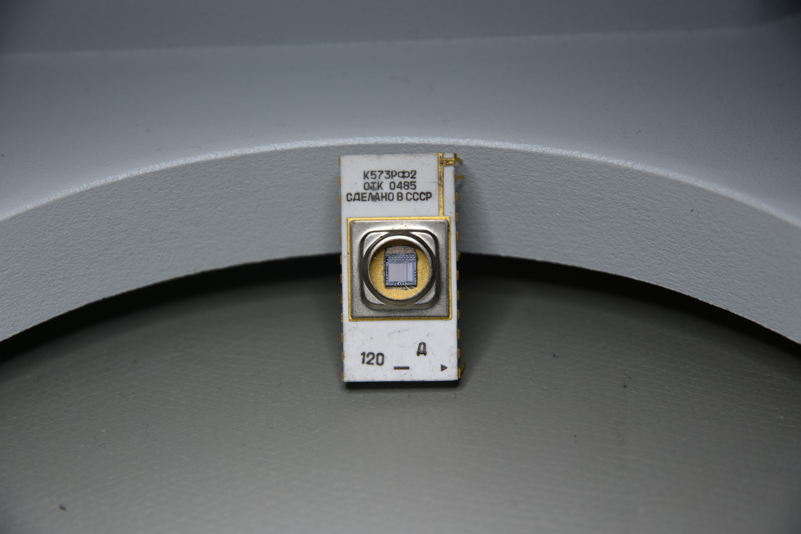
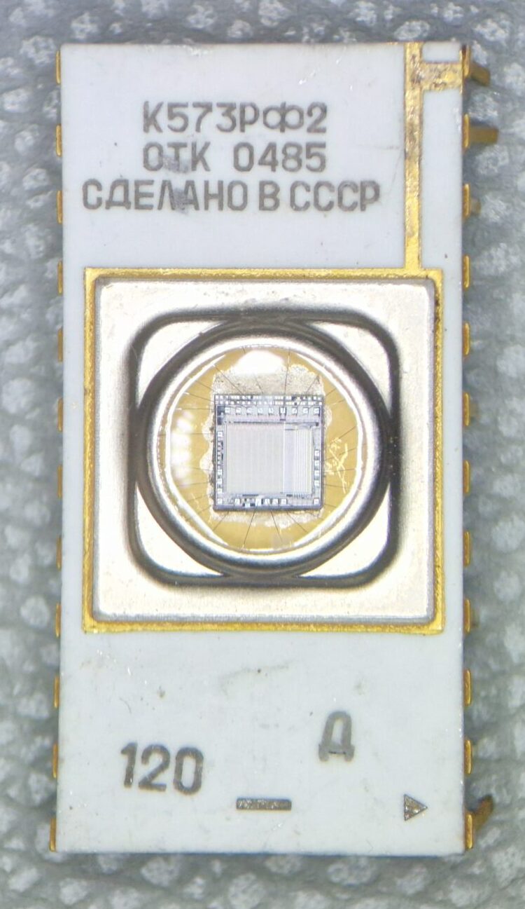
The recent dumpster diving dropped off few pieces of Soviet technology: a type K573RF2 EPROM. In original Cyrillic script it’s written as Κ573ΡΦ2 confused as K573PO2 or K573P02.
K573RF2 Soviet EPROM – Perspective View
K573RF2 Soviet EPROM
K573RF2 Soviet EPROM
Erasable Programmable Read-Only Memory (EPROM) retain data even after the power has been switched off. There is an interesting Wikipedia article on EPROMs which I’d like to refer to. EPROMs were used during the microcomputer era of 1970s and 1980s as non-volatile memory and have been replaced by modern memory types such as EEPROMs and Flash Memory. This particular integrated circuit (IC) from Soviet era is probably a clone of a 2716-type of EPROM which has been manufactured by Intel during the 1970s. The date code of this particular unit suggest a manufacturing date either in week or month 04 of the year 1985.
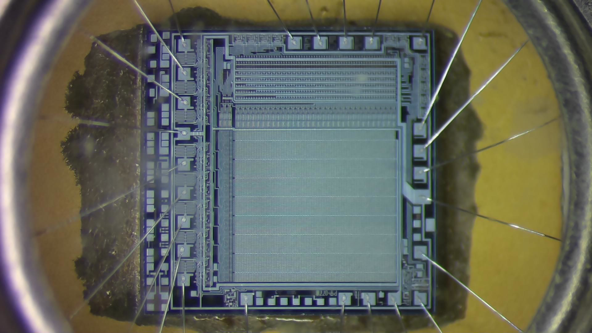
K573RF2 view on the integrated circuit
K573RF2 Soviet EPROM – IC view
I tried to get a good shot of the integrated circuit which can be seen through the quartz window. Unfortunately, I don’t have a suitable microscope with the necessary magnification optics to resolve more details. EPROMs have a distinct fused quartz window which permits to shine ultraviolet light (UV) on the silicon chip. UV light exposure erases the programmed memory cells which can be re-programmed again. Well, can’t say much about it. You can see the bonding wires and the arrangement of the memory cells. One could trace the bonding wires to the pin out and reverse engineer it. The packaging is probably made of alumina and with gold plated pins – this may indicate a military version of this IC?
I’ve found a datasheet for K573RF2 (K573P2-2716) and tried to translate it K573P2-2716_en via Google Translate. Have fun!
New addition to the lab! I bought Giovanni’s book via Amazon because it’s really epic. You can find freely downloadable, high-quality ebooks on his website: http://www.k100.biz/e-Books.html
Tektronix Epic Oscilloscopes by Giovanni Becattini. An epic book!
Unfortunately, it’s a “niche-topic book” but every vintage Tektronix aficionado will appreciate it. As an owner of 400, 500, 2400, 7000 and 11000 Series Tektronix Oscilloscopes, this book is just a must-have. Well-spent 70 EUR!
Thank you Gianni, your books are truly well-written, informative, beautiful and inspiring.
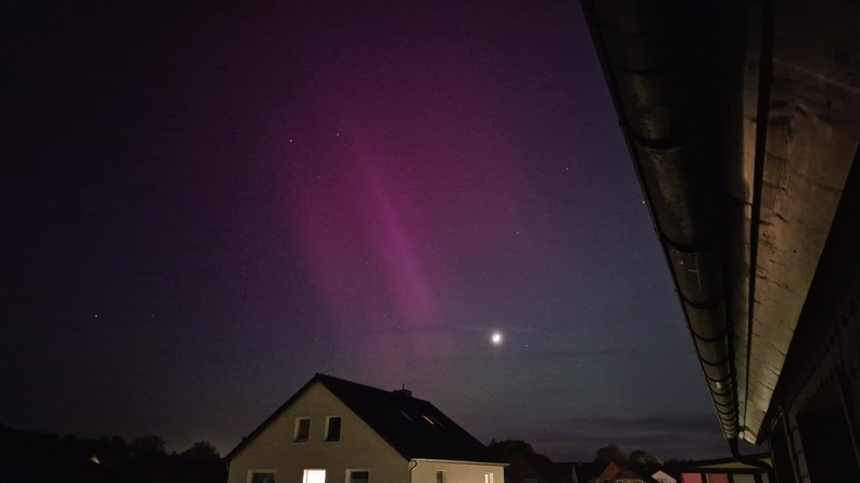
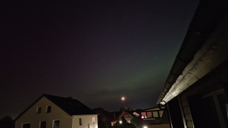
Earth got hit by a Coronal Mass Ejection from our Sun’s activity region AR3664 yesterday. Polar lights were spectacularly visible in most parts of Germany. My friend Michael woke me up around 23:30 CEST (= 21:30 UT) and I immediately rushed to the outside. After taking few (bad) pictures with my smartphone, I moved back to my apartment and observed the natural spectacle from my balcony. We even saw the International Space Station passing over us – a very eventful evening.
Visible Aurorae in Braunschweig, photographed with Samsung Galaxy S22 (2024-05-10): Image taken from the nearby street heading to the north. Unfortunately the street lights show some lens reflections
The geomagnetic storm isn’t over yet, we might be able to observe further polar lights tonight! I’ll try to catch some photographs with my DSLR camera!
Visible Aurorae in Braunschweig, photographed with Samsung Galaxy S22 (2024-05-10): Image taken from my balcony heading to the westVisible Aurorae in Braunschweig, photographed with Samsung Galaxy S22 (2024-05-10): Picture taken heading to the west
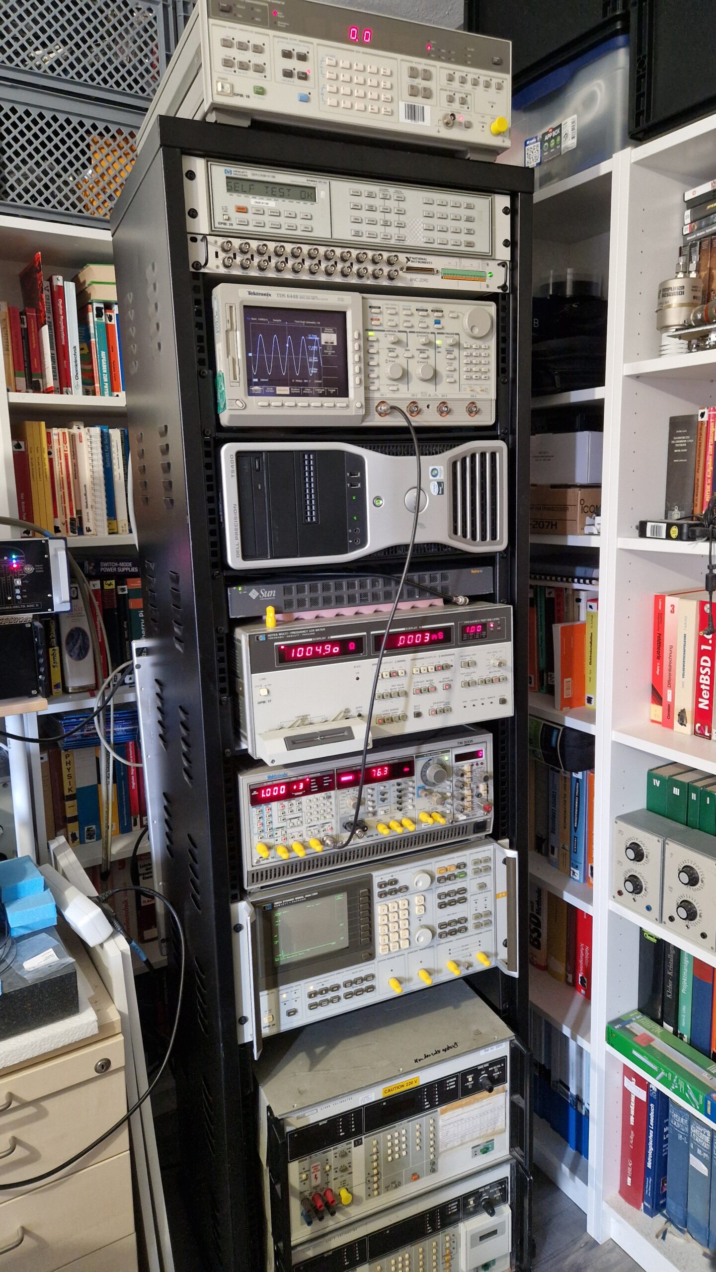
Yes, I have some kind of a Gear Acquisition Syndrome. Yes, I’m a Test Equipment Anonymous. Yes, I love Test Equipment! 🙂 However, this was bothering me for quite some time. The 19″ equipment was laying all over the place and I had some difficulties using it, since the instruments were bulky, scattered and there was no logical order as soon as I wanted to perform measurements. Luckily, a colleague of mine gave me a hint to buy a very cheap 19″ (42 HU) rack mount. This would solve few problems and also introduce new ones (more space for more equipment! Just kidding…). Anyways, I bought the rack mount and after few weeks of procrastinating, I finally equipped it with my 19″ sized test equipment. I’m pretty happy how it turned out. The most heavy parts are located at the bottom and lighter equipment is located at mid to top. It’s stable enough and won’t tip over and it can be easily moved around.
19″ Test Equipment rack mount.
Almost all instruments can be controlled remotely either via GPIB or RS232. An older Dell Workstation will be controlled via Windows Remote Desktop. Instruments from top to bottom are listed as follows:
HP 3325B – A 20 MHz frequency generator with some interesting features for audio testing
HP 3488A – Switch unit equipped with different modules. It’s used for automated, accurate and reliable signal switching or signal routing – it really depends on the used relay cards. I got few of them over the past years, e. g. types 44470A (10 CH multiplexer), 44471A (10 CH general-purpose relay module), 44472A (dual 4CH VHF switch module), 44473A (4×4 Matrix switch) and 44474A (16 bit digital I/O)
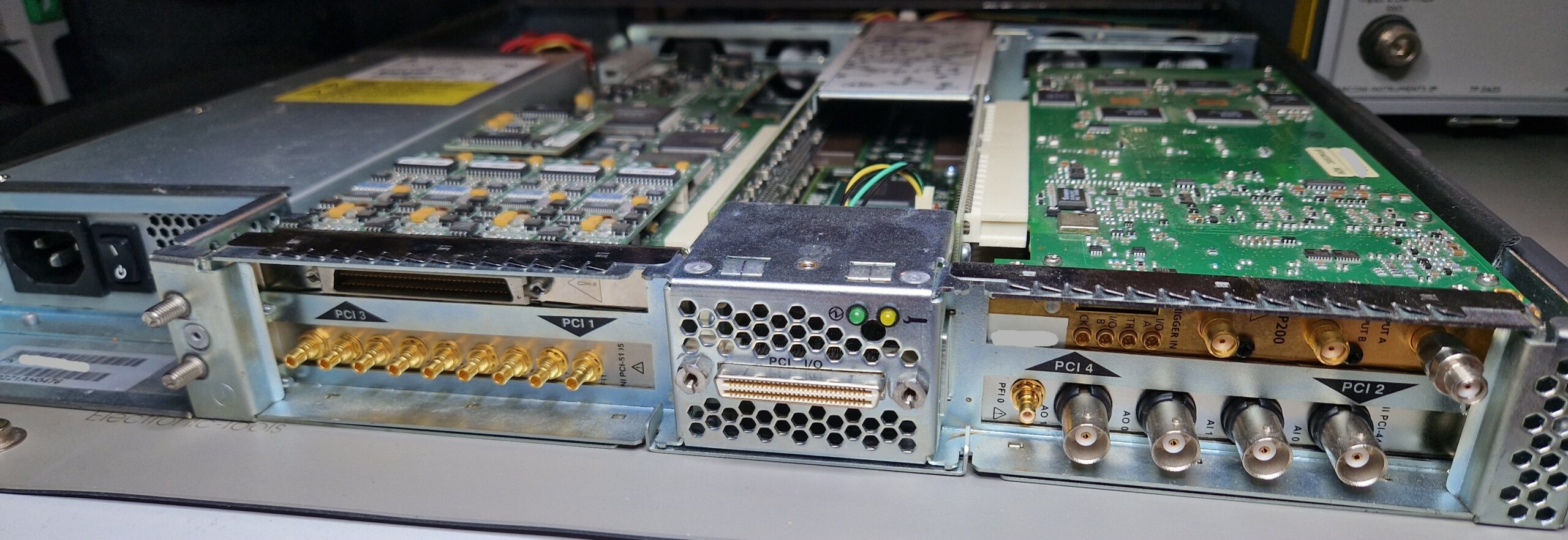
NI BNC-2090 is coupled with NI PCI-6110 (PCI multi-function-I/O-card with 4 analog inputs (12 bit, 5 MS/s per channel), 2x analog out, 8 digital I/O)
Tektronix TDS 644B, 4 CH, 500 MHz, 2 GS/s digital real-time oscilloscope. It’s a bit overkill for my audio-type applications – an excellent instrument for displaying waveforms, even RF stuff. A very useful feature is a GPIB interface for remote control and screenshot hardcopy (no need to use the disk drive)
Dell Precision T5400 workstation PC. It’s a 2007 era workstation which I bought probably around 2010 as a second hand PC. I used it like… forever. It was replaced by a faster workstation back in 2020. I haven’t dumped it because of the DVD burner and slots for 3x PCI and 3x PCIe cards. This makes it very valuable when it comes down to using data acquisition PCI cards from early to mid 2000’s era with a Win 7 or Win 10 operating system. Unfortunately this unit consumes a lot of power – it tends to heat up and it’s having thermal management difficulties during hot summers. Few of the ECC SD-RAMs failed over the past years but luckily they have been replaced easily. I tried to equip the three PCI slots with my oscilloscope cards, however, there were some serious thermal issues. I didn’t want to fry the cards so I put them inside of an external PCI expander system
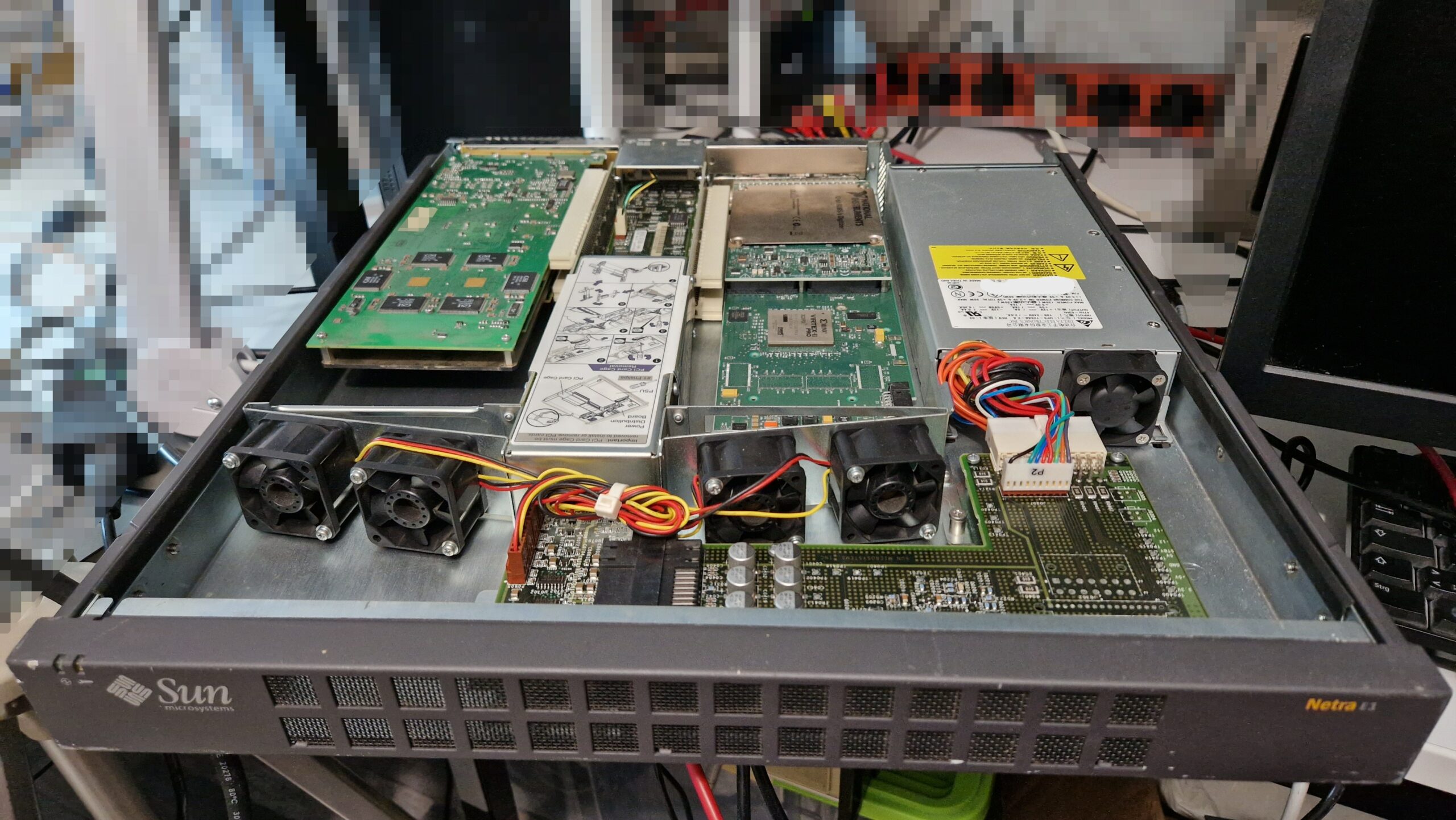
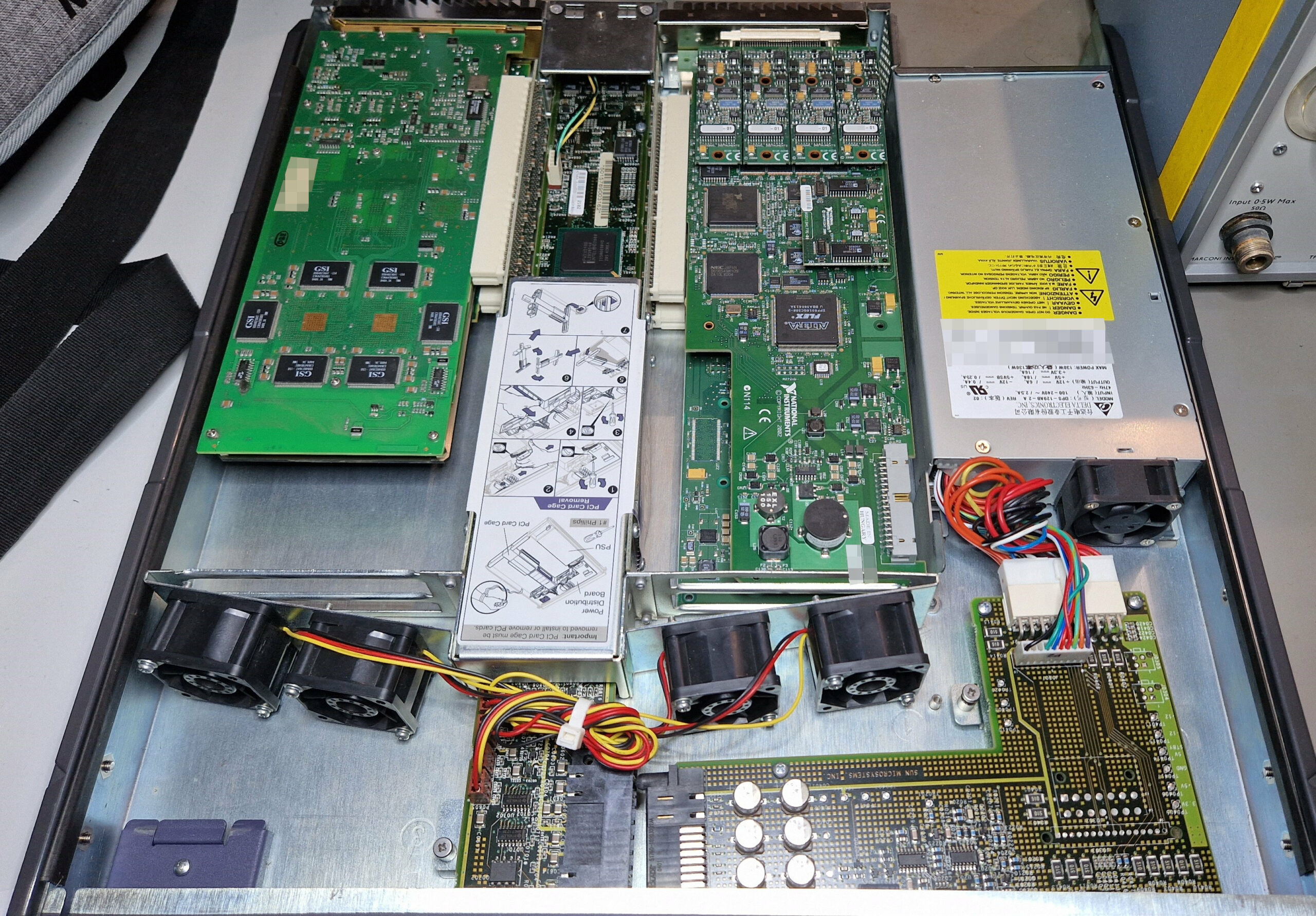
Sun Microsystems Netra E1. After having thermal issues and space problems inside of the Dell T5400, I was looking for a better solution to put the cards in a separate chassis and operate them via a PCIe/PCI bridge. Few solutions exist today, however only few are viable due to hardware/driver compatibility or power delivery constrains. The cheap expansion cards (mostly from China) can’t always deliver the 25-75 W of power to the oscilloscope card. In my case, as soon as the oscilloscope card demanded more power, the PC system crashed. After browsing eBay and looking for National Instruments’ “PXI-like” external chassis solution, I found Sun Microsystems’ Netra E1 as a viable option – however, the price was hefty. In retrospective, I’m glad I bought it because it was ready for use and it saved me a lot of time and trouble. The installation was super easy as PCI/PCIe bridge drivers exist at least since Windows XP. A downside of Netra E1 are the really loud fans. They work relentlessly at full speed; however, they keep the power-hungry cards at acceptable temperatures around 50-60 °C in comparison to 75-80 °C inside of Dell T5400!
Sun Microsystems Netra E1 – PCI Expansion System
Sun Microsystems Netra E1 – Top view.
Sun Microsystems Netra E1 – Back view.
Unfortunately, Netra E1 is obsolete technology and no replacement parts exist on the 2nd hand market. Those units were produced around the year 2001 as an expansion system for Sun’s Netra Servers. I might be wrong about this but IIRC their PCI expansion product line was acquired by a company called MAGMA somewhere around mid 2000’s. MAGMA was specialized in building PCI Expander Systems for the Pro Tools Digital Audio Workstations (Pro Tools by Avid Technology, famous tor their audio/video editing software). eBay has some offers with MAGMA expansion chassis up to 16 PCI card slots, however they come at an unrealistic price of $500 to $1000, at least for a hobbyist budget. Anyways, beside the three existing PCI slots inside of the Dell workstation, I was able to put all of my four “power hungry” PCI cards (full length) inside of the 19″ chassis
NI PCI-6110: multi-function I/O card
NI PCI-5105: 8 channel, 12-bit, 60 MS/s digitizer/oscilloscope with up to 60 MHz analog bandwidth
NI PCI-4461: dynamic signal analyzer, basically a $10k sound card, still produced today – according to NI, it can be bought until 2024-12-31!
Agilent/Acqiris AP200: 1 channel, 500 MHz, 2 GS/s high-speed digitizer/averager card (used in radar tech or mass spectrometers)
Yokogawa/HP 4274A Multi-Frequency LCR Meter. I have a bunch of HP fixtures for components, unfortunately the LCR meter needs a repair. Should be hopefully an easy fix since the errors appear after warm-up. Fun fact: The Japanese government was very restrictive and protected their markets in the early days. In order to enter the Japanese market, companies from foreign countries such as United States were obliged to “team up” with a local Japanese manufacturer so they could sell their products in Japan. I guess HP teamed up with Yokogawa and Tektronix had a partnership with SONY. That’s the reason why there is occasionally a double company logo on some pieces of test equipment.
Tektronix TM5006 chassis equipped with
Tektronix FG5010, 20 MHz frequency generator (GPIB-controllable)
Tektronix AA 5001, audio analyzer capable of measuring Total Harmonic Distortion (THD), also GPIB-controllable
Tektronix SG505, audio frequency generator with exceptional ultra-low distortion sine-waves, perfect for audio amplifier testing
Tektronix DC 503, digital counter (doesn’t work, needs a repair)
HP 3562A Dynamic Signal Analyzer. A very capable FFT analyzer e. g. for audio and vibration testing and frequency response analysis in the µHz … 100 kHz regime
Fluke 5100B/5101B Calibrators. They can provide AC and DC voltages and currents and also resistances for calibration of up to 5.5 digit DMMs. Unfortunately, both need repair (power supply issues). Currently they are not in use – I’m hoping to repair them either later this year or maybe in early 2025
Surrounded by the rack mount are my book shelves with many books about physics, chemistry, operating systems and other stuff. A HPM 7177 digitizer can be seen at mid-left. There are only three cables left which are connected externally to the chassis: 230 V power, GPIB and Ethernet. I could replace GPIB with an NI GPIB-USB and Ethernet with WiFi. This would of course simplify the cable management but I’m very happy how everything turned out. I’ll need to find some lifting feet for the rack mount since it’s a bit overloaded with ~200 kg of equipment and it could cause damage the floor and the wheels over time.
Most of the test equipment seen here has been acquired during the past 3-4 years. Some pieces were really cheap (< 100 EUR), others rather expensive (> 300 EUR). It will be used for my laser interferometer and accelerometer calibration project which I plan to build in the future.
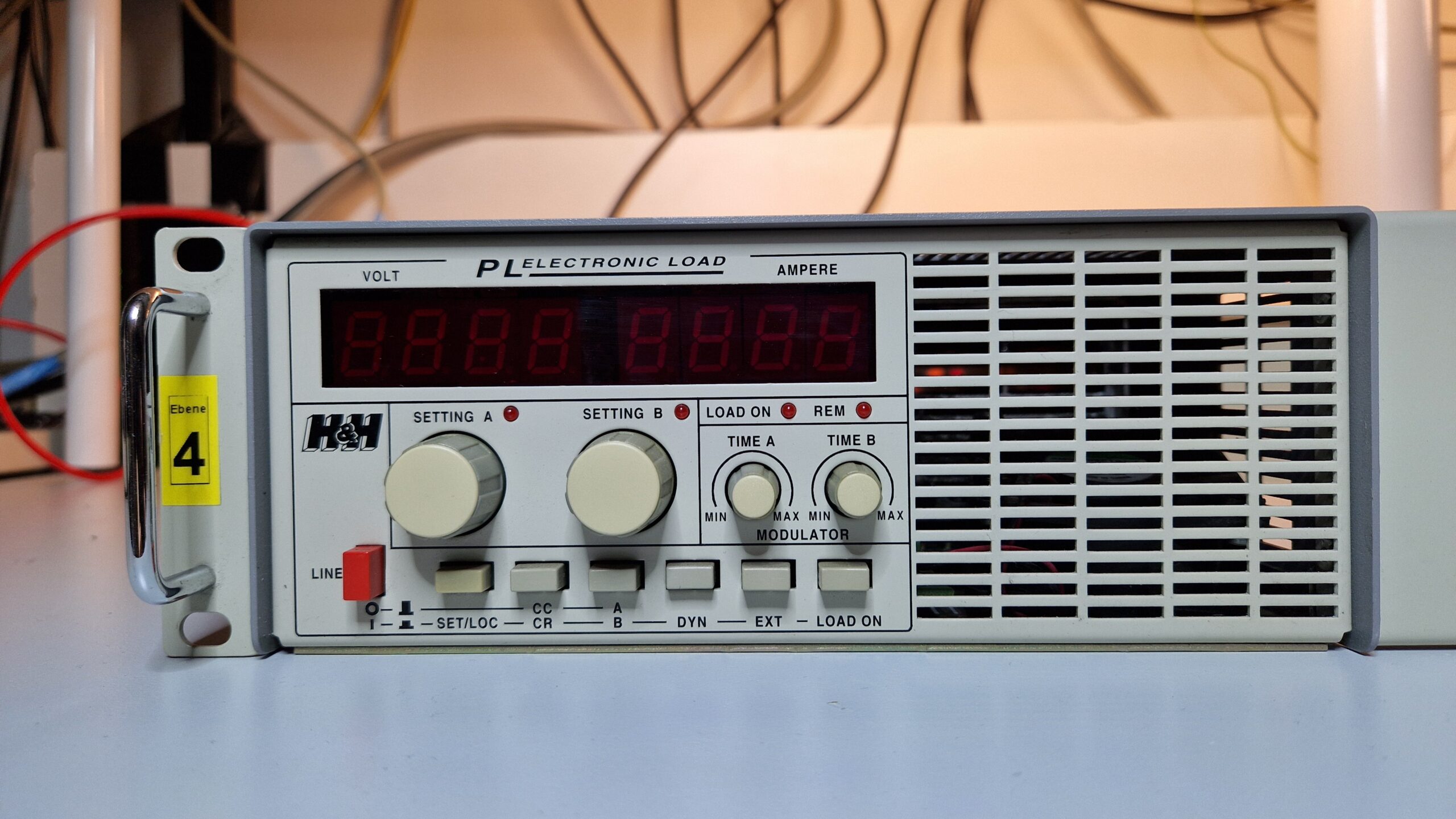
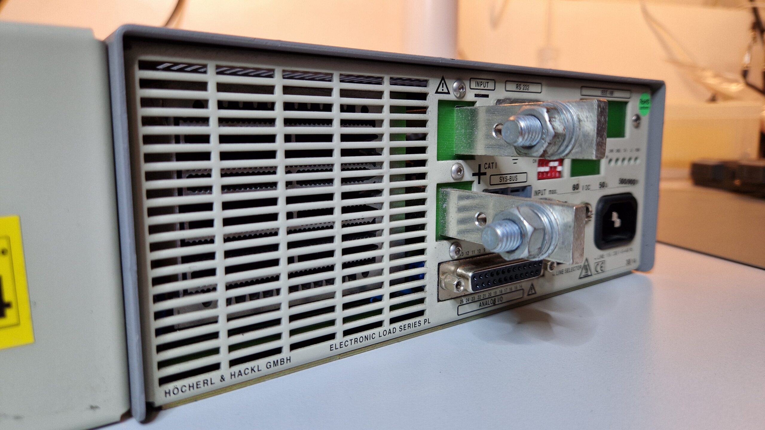
I bought a Höcherl & Hackl PL506 DC electronic load just recently. It’s a nice piece of equipment to test switch-mode power supplies (SMPS) or any DC power sources like solar modules or batteries. I will need few of those for Tektronix SMPS repairs. As far as I can tell, DC electronic loads are rather rare and expensive units. So I grabbed one on an auction site for a very decent price compared to current offers (which is crazy, they ask 600…1000 EUR for such unit).
Höcherl & Hackl PL506 front panel.
Höcherl & Hackl PL506 back side.
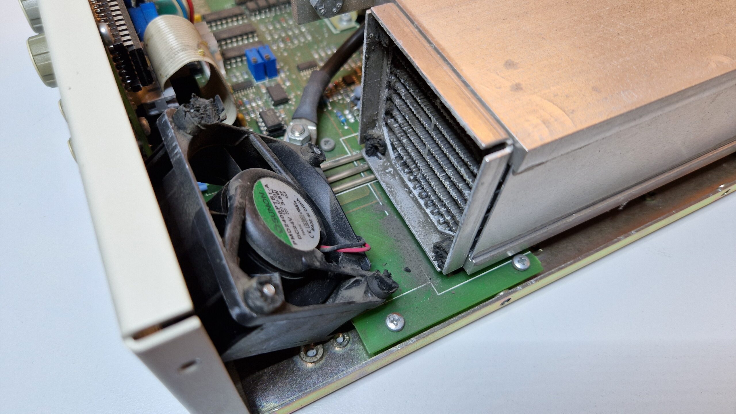
After unboxing and shaking the unit, I noticed a strange noise. Since it’s easter holidays here in Germany, I thought it was some kind of a “Kinder Surprise Egg” time!
But no, I was disappointed. No easter eggs 🙁 It was the fan which broke off. I looked for other damaged parts and defects but there were none. No signs of burned parts, bad electrolytic capacitors etc. Looking good inside!
Höcherl & Hackl PL506.
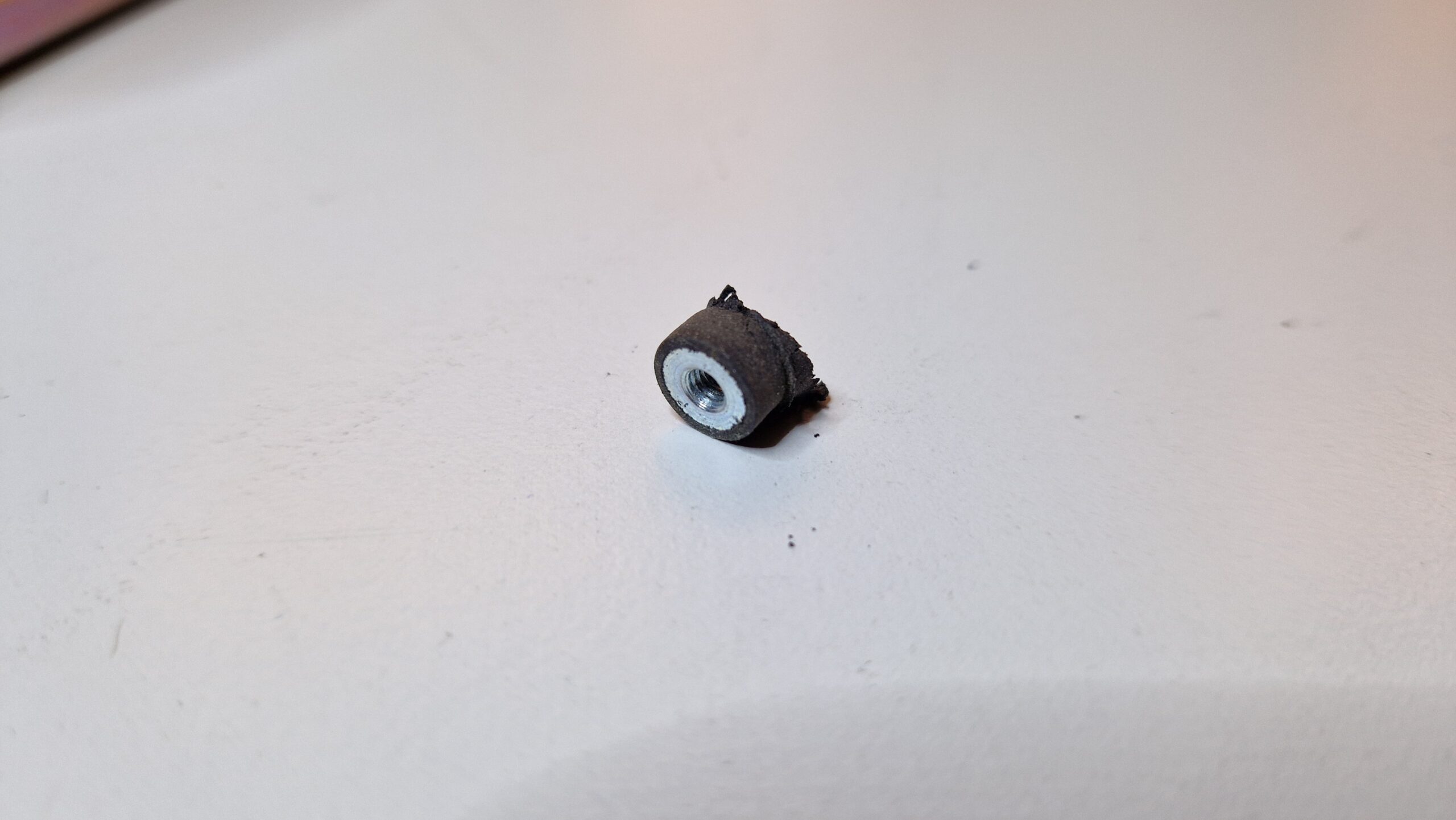
H&H PL506 – The unit was shipped like this. The rubber vibration isolators broke and the fan fell off.
The vibration isolators probably became brittle over the years and broke during the transport. The fan fell off and had to be reattached. The front panel buttons are a bit crusty, too and will need to see a maintenance one day. The heat sink could need a clean-up, too. Build-up of dust and dirt diminishes heat transfer and can cause either performance issues or overheating of power dissipating MOSFETs.
Rubber dampener with metal thread insert.
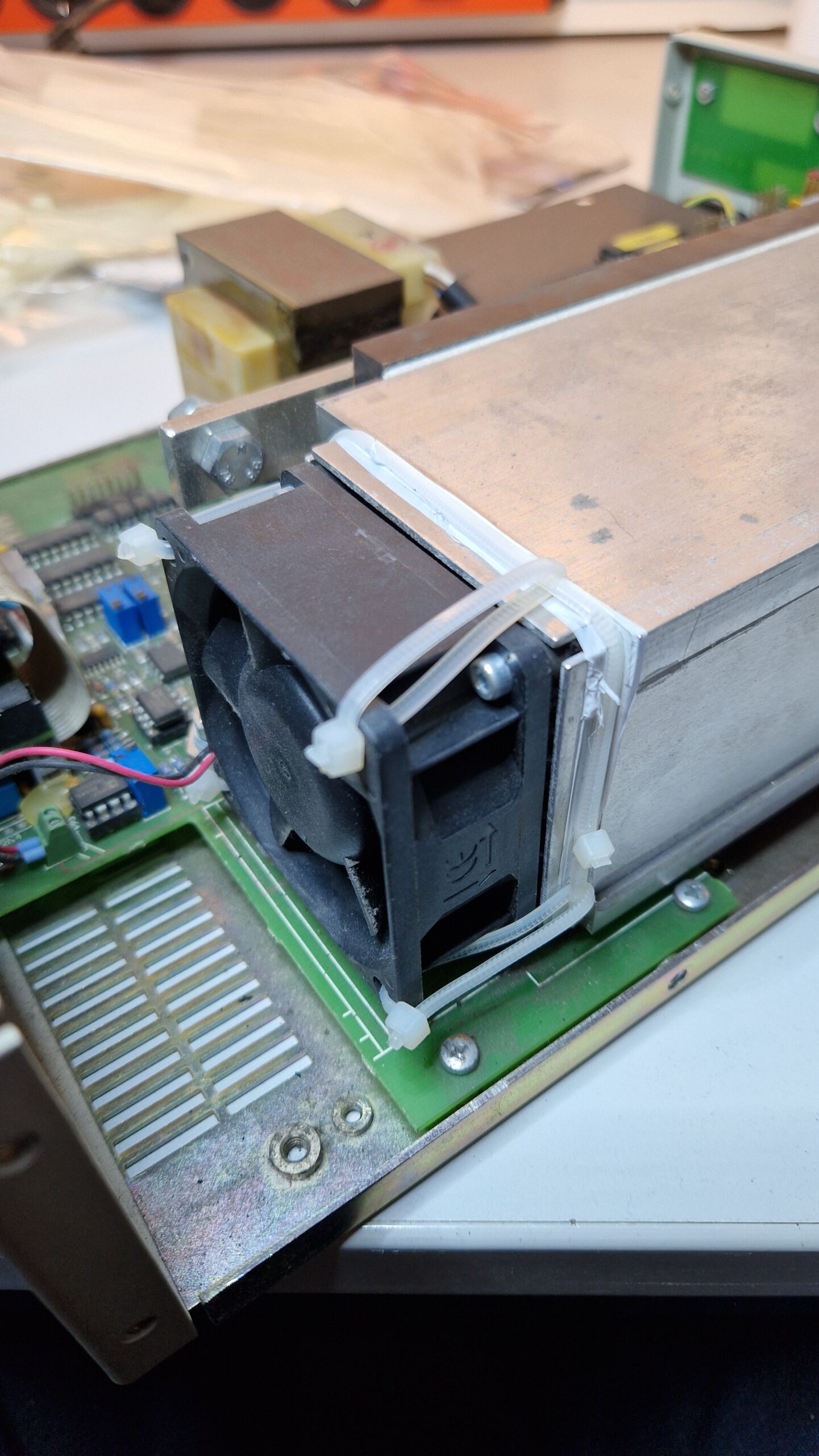
I was looking for a suitable replacement in my electronics parts bins but found nothing. I used zip ties to reattach the fan to the heat sink. The unit was fixed in less than 10 minutes.
Problem was fixed with zip ties.
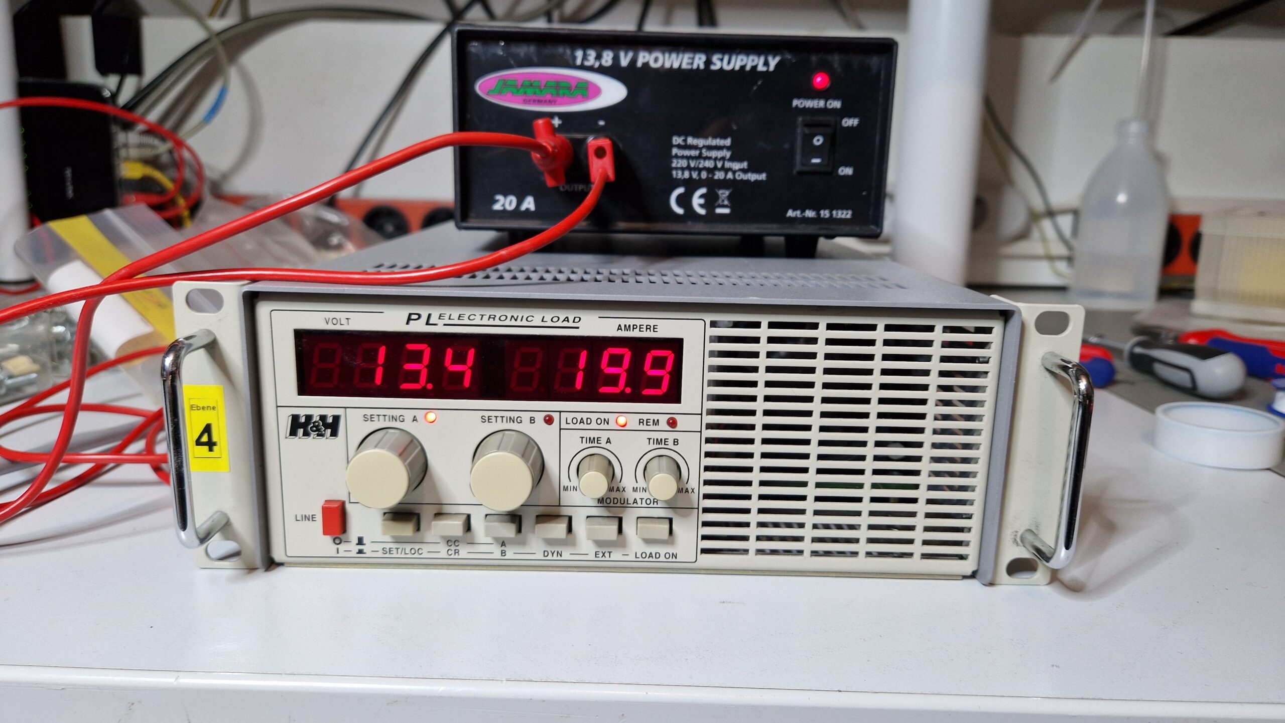
A quick test with a random 13.8 V SMPS was successful. I was able to load 19.9 A at ~13.4 V which corresponds to ~267 W output power of the SMPS. This DC electronic load is capable of dissipating 500 W continuously or up to 900 W short-time. This was a short-time test with 4 mm banana cables since I didn’t have proper high-current cables at hand.
Höcherl & Hackl PL506. Testing a 13.9 V / 20 A power supply.
Very nice addition to the lab. Hope this will be useful for future repair and maintenance projects!
Tektronix TDS 3034B four channel color digital phosphor oscilloscope.
A “new” oscilloscope arrived in the lab just recently thanks to my friend Matt, who relayed the offer to me. It’s a wonderful instrument from the early 2000’s era: a Tektronix TDS 3034B Four Channel Color Digital Phosphor Oscilloscope. The oscilloscope’s analog bandwidth is specified at 300 MHz with a sample rate of 2.5 GS/s per each channel. It has a ton of options (e. g. FFT, 3LIM, 3TRG) and a communication module with VGA monitor output and GPIB/Ethernet/RS-232 for communication and control. There is also a battery compartment, however, the battery was not included. The “Waveform Intensity” knob simulates the intensity control of an analog oscilloscope with a cathode ray tube – therefore a “Digital Phosphor Oscilloscope” or DPO. The size of the oscilloscope is very convenient and perfect for a desk use – doesn’t take much space and it’s fast and responsive compared to my older Tektronix TDS 754D oscilloscope.
Tektronix TDS 3034B back side with battery/probe compartment.
I was able to set up the communication to my PC via GPIB (IEEE 488). Since I already had the Tektronix WaveStar Software for Oscilloscopes installed on my Windows 10 PC, I was able to quickly transfer screenshots/hardcopies, measurement data and sample data from the instrument to my PC. No diskettes or USB drives were needed. It is possible to control the oscilloscope remotely which is absolutely fantastic for measurement documentation and measurement automation purposes! It’s a great addition to the lab and it will serve to me as my daily workhorse among other oscilloscopes, of course.
Tektronix WaveStar for Oscilloscopes. Easy way to transfer screenshots and data from Tek TDS 3034B to a Windows PC.
Bandwidth Upgrade
It seems to be very common (even nowadays in 2024) that the oscilloscope manufacturers design a generic oscilloscope parts which can be used for different models. The oscilloscopes are then assembled with similar to identical hardware components (presumably because it’s cheaper manufacturing-wise) but the measurement capabilities are determined either by hardware (jumper settings) or by software (locked/unlocked options). For example, Rigol DHO 800/900 Series Oscilloscopes can be upgraded from 70 MHz to 100+ MHz via software. Thanks to Matt, he gave me a hint that the guys at EEVblog have figured out how to perform an upgrade of the Tektronix TDS Series oscilloscopes to different models. So already having an excellent 300 MHz & 2.5 GS/s oscilloscope at my fingertips, I was curious if I could upgrade it to the 3064B model which has 600 MHz analog bandwidth and 5 GS/s sample rate. I tried out the EEVblog’s upgrade procedure and it seemed to work without bricking the oscilloscope. I’ll just quickly summarize the procedure here.
*IDN? query via GPIB.
Tektronix TDS 3034B boot screen.
Boot up the device and set up the communication via GPIB (e. g. GPIB address and talker/listener mode). Connect the device to your GPIB controller
I used the National Instruments GPIB-USB-HS controller device along with current NI’s GPIB drivers (driver version doesn’t matter much, you could also use the VISA drivers from Keysight, Tektronix or Keithley). The TDS 3034B Firmware Version was v3.39
The communication between the PC and the oscilloscope was established with NI Measurement & Automation eXplorer’s (NI MAX) own GPIB Instrument Communication. I guess you could use any GPIB communication software, e. g. pyvisa for Python
Check whether the oscilloscope responds to the *IDN? query. If yes, proceed, if not – try to find the problem and fix it (obviously)
Send the following commands to the oscilloscope PASSWORD PITBULL MCONFIG TDS3064B
Just send (write) the commands in the order as shown above! Do not use a “GPIB query” since there will be no response action from the oscilloscope. Upper/lower case letters don’t matter.
Now power-cycle the oscilloscope (turn it off, wait few seconds and turn it on again). It should boot up with a new screen and new model. If it doesn’t show the new model, something went wrong with command transmission via GPIB. As far as I could tell, some models accept only different MCONFIG-commands, such as “MCONFIG TDS3054” without the letter “B” at the end. Anyways, after sending the commands via GPIB and power-cycling the oscilloscope, it should show up with the new model
Changing the TDS model will result in an uncompensated waveform. I observed a DC offset and noise on my CH1 through CH4 waveforms post-update. The solution to this problem is quite easy: wait some time (at least 10-15 minutes) for a warm-up and perform the Signal Path Compensation (SPC), which can be found in the Utility → System Config → Cal
menu. This will perform an internal calibration where the noise and offset errors are compensated. The oscilloscope should be ready for performing measurements afterwards
*IDN? query after BW upgrade.
Boot screen after BW upgrade.
Waveform pulse post-upgrade. Sample rate is at 5 GS/s.
Tek’s Signal Path Compensation.
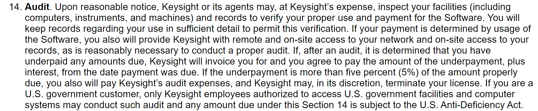
That’s how it worked out for me. It took me just few minutes to convert a Tektronix TDS 3034B into a TDS 3064B. I’d recommend to check out the linked EEVblog thread for further information on the TDS 1000/2000/3000 Series upgrades. Of course I can’t be held responsible if you try it out and damage your instrument (e. g. calibration data or warranty is lost or the device is bricked) since I’m sharing this information and tried it out on my own oscilloscope. This is solely done at one’s own risk! Please be careful when trying out this procedure and please read the EEVblog thread prior to changing the instrument. Always make backups of your oscilloscope firmware prior to changes. Also hacking the device in order to use unlicensed software options is… well… “illegal”… I guess… Keysight’s Agents will hunt your PC down! 😉
Excerpt taken from the Keysight N1500A EULA. This is not a joke (well, it’s a well-known meme), see it for yourself: https://helpfiles.keysight.com/csg/N1500A/License_Agreement.htm
Checking the Oscilloscope Analog Channel Bandwidth
I did some initial bandwidth testing with my Leo Bodnar Fast Risetime Pulse Generator. The pulser generates repetitive 10 MHz square waves (~1 Vpp) with a rise time of around (30 ± 2) ps. It can be used to easily test the oscilloscope’s analog channel input bandwidth. The analog bandwidth of an oscilloscope can be calculated as follows:
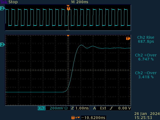
So a measured 10%-90% rise time of \(t_r = 1.000 ~\mathrm{ns}\) results in an analog bandwidth of \(0.35/(1.000 \cdot 10^{-9} ~\mathrm{s}) \approx 0.350 \cdot 10^9 ~\mathrm{Hz}\) or 0.35 GHz which is basically 350 MHz. So prior to the bandwidth upgrade we were expecting an oscilloscope bandwidth of ~300 MHz at a 2.5 GS/s sample rate, post-upgrade it should be around ~600 MHz and a 5 GS/s sample rate. I’ve measured the rise time of all four channels in order to see if there are any significant differences between them. The oscilloscope settings were as follows: Coupling: DC, Termination: 50 Ω, Trigger: External, Acquisition Mode: 64× average per acquisition at 10k points and 5.00 GS/s. The trigger was delayed by approx. -10 ns.
Tektronix TDS 3034B CH1 risetime.
Tektronix TDS 3064B CH1 risetime.
Tektronix TDS 3034B CH2 risetime.
Tektronix TDS 3064B CH2 risetime.
Tektronix TDS 3034B CH3 risetime.
Tektronix TDS 3064B CH3 risetime.
Tektronix TDS 3034B CH4 risetime.
Tektronix TDS 3064B CH4 risetime.
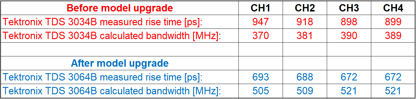
The measurement results are summarized in the table below.
Analog bandwidth calculations from measured rise times for each oscilloscope channel. Comparison between Tektronix TDS 3034B before model upgrade and after model upgrade to TDS 3064B.
As we can see, the full bandwidth of 600 MHz for a Tektronix TDS 3064B has not been achieved. However, there is a measurable improvement. Channels 3 and 4 seem to have a slightly higher bandwidth than channels 1 and 2. The rise time measurements deviate on each acquisition so I would estimate an uncertainty in the rise time measurements of approx. ±10 ps. I also wonder if the overshoot/undershoot calculations are correct. I’ll have to look into this manually, since the data samples can be exported in a CSV file.
Conclusion
Nevertheless, the bandwidth upgrade was successful! 500 MHz analog bandwidth at 5 GS/s is more than enough for my needs before stepping into the GHz time domain regime. And no need for a battery if there is a food compartment in your oscilloscope! Tested successfully with carrots! 😉
It’s currently cold outside (-8 °C) here in Germany and I skipped my cycling tour yesterday. Instead I got myself some stuff to play with during the cold and dark winter days.
Some new gadgets on the desk.
A “new” handheld oscilloscope Tektronix THS 720 (STD) appeared in my lab! It had a dead Ni-Cd battery so I replaced it with a new one. It seems to work, however, it also seems to have the usual aging issues with optocouplers. Channel 1 shows some DC offset while Channel 2 looks fine DC-wise. The price for this scope was really “OK” (<200 EUR), it’s great for troubleshooting switch-mode power supplies due to fully isolated oscilloscope input channels. It has a built-in multimeter to check voltages simultaneously – great tool for repairing broken test equipment! Well, this instrument also needs a repair, so it’s some kind of repairception? hmm
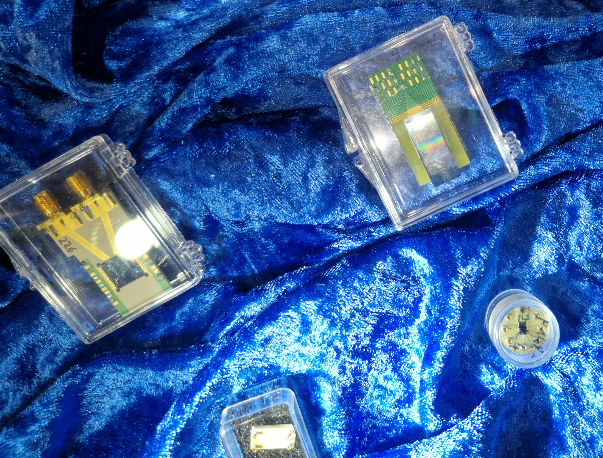
On the bottom right, we have four Sprague TANTAPAK® wet slug tantalum capacitors, 820 µF, 20-30 V(DC) each. If they haven’t been abused and aren’t leaky, maybe they will be used as decoupling capacitors for a nanovolt noise measurement of a LTZ1000ACH. Need to be tested for their capacitance, ESR values and leakage current. See Jim Williams’ work on Linear Technology Application Note 124. A HP 10514A mixer can be seen on bottom mid. Bought it out of curiosity, will test it. Top left shows a 10 MHz OCXO for a HP 53131A type of frequency counter. On the left hand side, a SUNSHINE IC socket fixture can be seen. A friend told me it was used along with an ancient SUNSHINE EPROM programmer PC card, the one with an 8-bit PC/XT-bus maybe?
Bottom left shows a Raspberry Pi 5 (8 GB) with a cooling fan. Raspi5 was announced in November 2023 but I couldn’t buy it in online shops because there were none available. It took them almost 6-7 weeks to restock their supply. I didn’t want to pay high prices for a Raspi 5 on second hand markets because the offers were 30-50% overpriced in the order of 130 – 150 EUR (which is crazy!). Will be a nice upgrade to my Raspi 3B standing army. I’ve ordered some accessories such as a cooling fan, the 27 Watt USB-C Power Supply, a black case, RTC battery, Micro HDMI adapter cables and a microSD card.
Raspberry Pi 5 8 GB.
And there is a possible repair project on the horizon. A HP 3458A has presumably lost its calibration data due to a dead battery of the Dallas DS1220Y-150 Nonvolatile-SRAM. The NV-SRAMs in a HP 3458A store settings/preferences and calibration constants. As long as the unit is powered up, the battery coins inside of the Dallas ICs aren’t discharged. However, once the digital multimeter is turned off for a longer periods of time (e. g. months, years), the battery is slowly discharged. Unfortunately, the discharge curve of a NV-SRAM does not show any signs of discharge when measuring its voltage – instead the battery voltage drops suddenly below a power-up threshold and all stored data is lost. The life time of the battery can last between ~8 up to 30 years and it strongly depends on environmental and usage factors. Therefore: please do backup of your IC contents in order to prevent a potential nightmare.
After power up, “RAM TEST 1 HIGH” message appears. With some luck, the batteries of the calibration data NV-SRAMs may be still alive…
HP 3458A is a famous example but there are also oscilloscopes out there (e. g. Tektronix 2465B/2467B, older TDS Series) with a memory-loss time bomb. I’m currently taking care of ordering replacement NV-SRAMs and will try to revive the unit.
HP 3458A Dallas Nonvolatile SRAM. The DS1230Y NV-SRAMs store the preferences and settings while the DS1220Y-150 type holds the calibration data. If the internal battery of this chip dies, the calibration constants will be lost and the instrument will be out of spec. It will need a full recalibration.
HP 3458A A1-9530 board inspection.
I’ll resume my cycling efforts tonight. It’s no pleasure doing this at -8 °C mostly because of cold wind blowing into the face for about an hour or so. Nevertheless, there is no bad weather, only bad clothing!
The new year is already 5 days old. Nevertheless, happy new year to everyone who reads this blog. As always, I’ll try to post on a regular basis about my adventures in the fields of bike touring, amateur radio and test equipment / gear acquisition syndrome. Keep up the good work, may your projects be fulfilled in 2024. Stay healthy and sound and keep up a positive attitude.
73, Denis (DH7DN)
Hiroki test lead with a rather dangerous adaption 😉
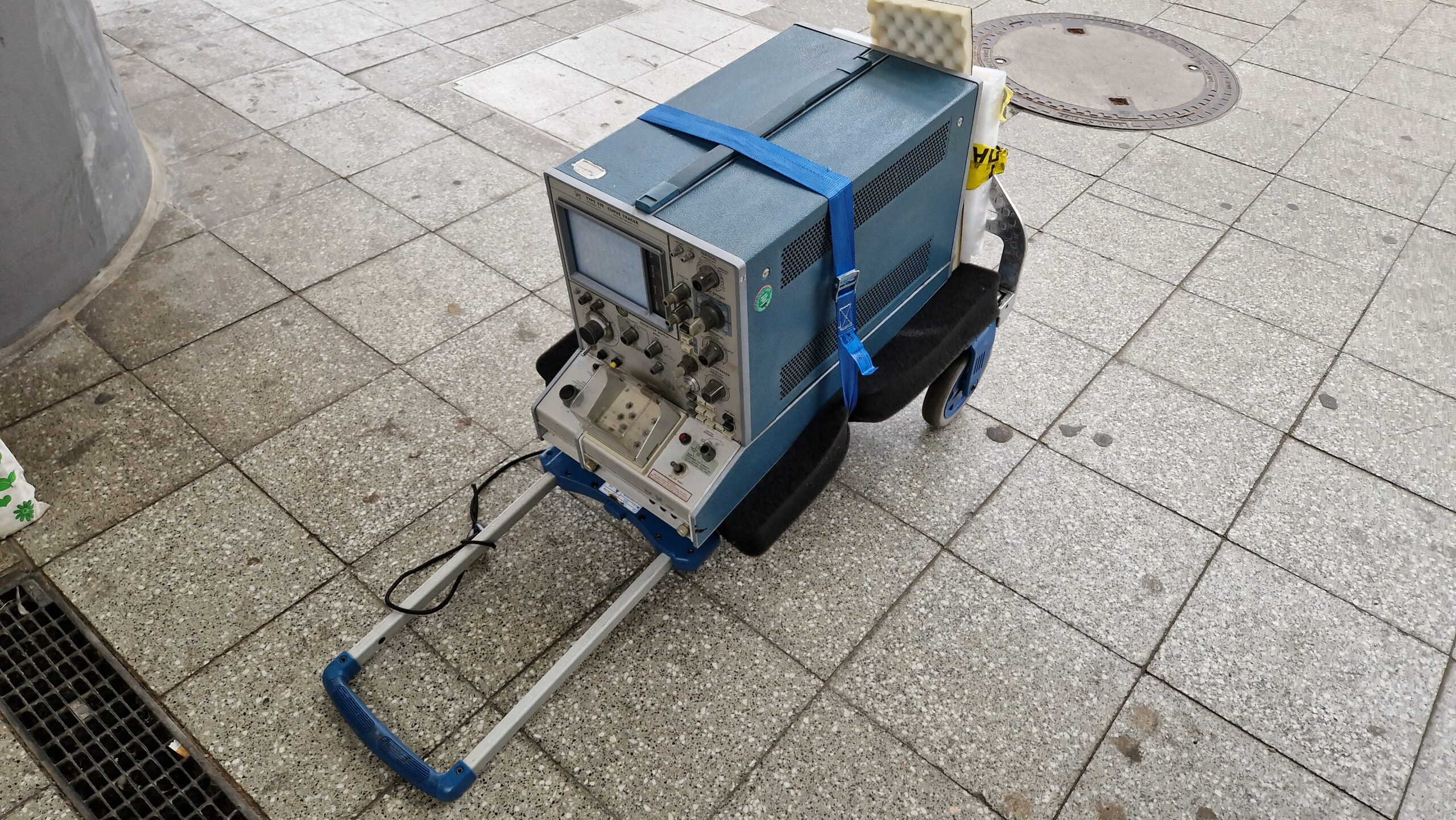
I bought a Tektronix 576 Curve Tracer on the second hand market some time ago. Unfortunately, the seller wasn’t able to ship it and he did not live in my region. The pick-up place was near the town of Düsseldorf – a 350 km distance from my place. Oh boy…
The problem with this particular curve tracer is its size and weight: it can’t be hand-carried for long distances because it’s a 35 kg (~70 lbs) chonker. Even if it’s carried by one person, one has to be very careful not to damage delicate parts and also for health and safety reason when carrying heavy instruments in a wrong posture. Shipping this curve tracer via regular parcel service is almost impossible or very expensive. Since I don’t have a car right now and car rentals are also very expensive, I tried to pick it up and bring it back home by train. The idea was to use a small hand truck for transportation in busses and trains. This way, it should be possible to treat it as luggage.
Well, it kinda worked out somehow! I started my journey in Braunschweig at around 8 am and headed towards the central train station by public transport. Luckily the connecting trains were on time so I reached Düsseldorf at 12 pm. The seller was very kind and agreed to meet at the nearest train station where he handed over the curve tracer with a manual. It took me about 20-30 minutes for packaging and securing the curve tracer with straps.
The Tektronix 576 Curve Tracer was handed over to me on a parking place near Düsseldorf.
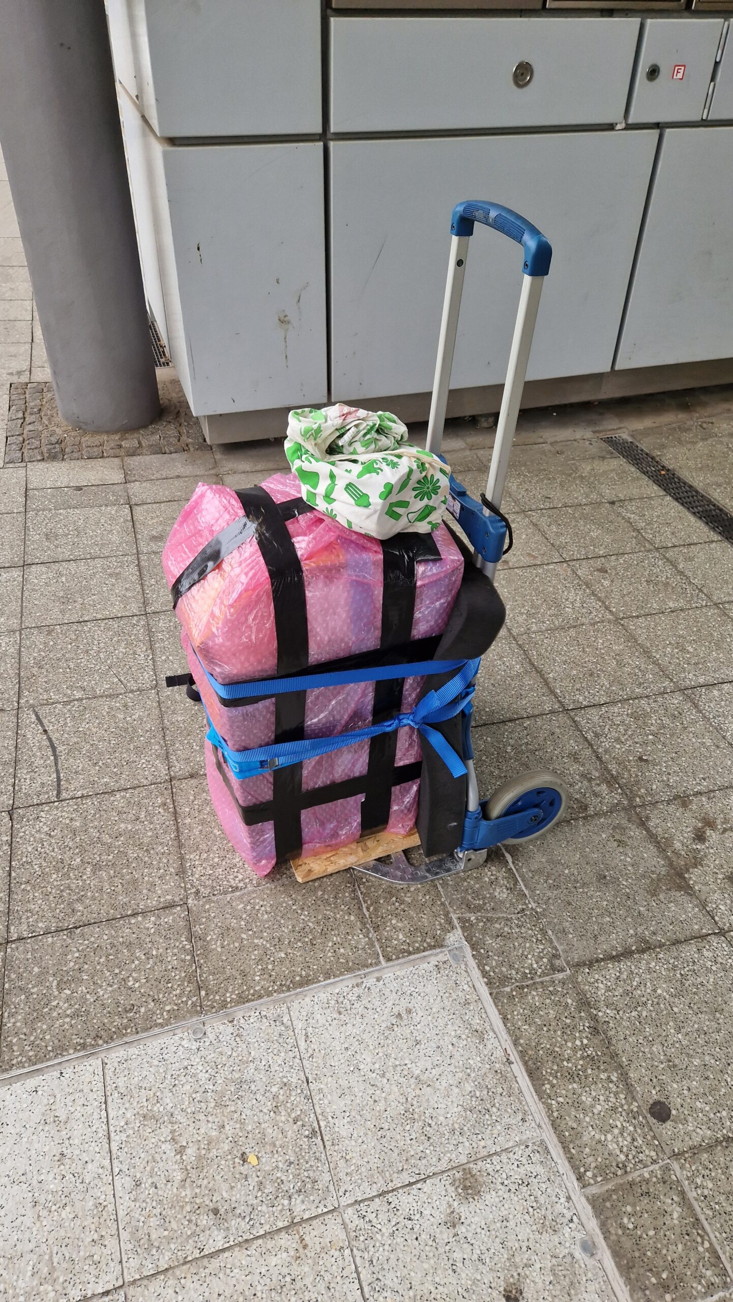
Quick and dirty transport in order to escape the rain and get to a dry spot.
Tektronix 576 properly packed on a train station.
The journey back from Düsseldorf to Braunschweig was much more difficult and was delayed multiple times. However, time was not an issue and I managed to get back home with a 2 hours delay at 7 pm. The total price for travelling by train in both directions was around 70 EUR which is comparable to current gasoline prices for a ~700 km route.
The curve tracer fits very well inside of the luggage compartment.
Some trains were full and crowded.
We had bad weather on this day. However, the Tek 576 was well protected from rain.
I used some cardboard pieces and soft foam to protect the knobs and sensitive parts. Hard foam was used to protect the back side and a grey soft foam mattress was added for additional cushioning. The bubble wrap was used as thermal isolation and rain protection (temperature shocks aren’t good for electronic and plastic parts). The straps were used to secure the instrument so it doesn’t fall over. The blue masking tape is really useful for attaching the cardboard to the housing. The masking tape is very easy to remove without leaving tape residue or peeling off the paint.
Unpacking of the Tektronix 576 Curve Tracer back at home.
Tektronix 576 Curve Tracer taking place at the Tek Cart.
After getting back home, it took me some time to unpack the Curve Tracer. I’ve waited at least 24 hours to power up the unit since it had to acclimate to the ambient temperature. It’s not a good idea to power up a cold instrument which has been exposed to low temperatures for hours. I was very tired after the travel but everything seemed to work out very well.
I couldn’t find any broken or damaged parts. Taking a look inside of the instrument showed no signs of a transport damage. From my experience, such a delicate instrument needs to be handled properly, you can’t always trust the parcel service. Taking care of the transportation is the only way to ensure the instrument will “survive” the move from A to B. Who else didn’t experience the “Courier Transformation” at least once in their life? By the way, it’s a nice pun to the “Fourier Transformation” 😉
As you can see, heavy instruments can be transported by train, at least here in Germany. However, this transportation method becomes very impractical as soon as the round trip times exceed 12-13 hours. Travelling 12+ hours by train is no fun for sure therefore it’s not always a viable method.
That’s it for today. The next blog entry will show some post-power up experiments and shots of the Tektronix 576 innards.
I don’t consider myself as a voltnut. I don’t design precision circuits and I don’t do crazy and expensive things like selecting, binning or matching of super-expensive components (Zener voltage references, foil resistors or opamps). I don’t spend my evenings on Christmas doing circuit simulations in LTspice. However, I like the idea of DIY-ing of an existing precision circuit design and verifying its performance. Thanks to Illya Tsemenko, Marco Reps and the voltnuts all around the world and their endless efforts in searching for the best design for a DIY voltage reference – it is nowadays possible to build a laboratory-grade, high-performance solid state voltage reference using off-the-shelf components which performs very close to their commercial available counterparts and costs just a fraction of its price (perhaps less than 10%). In this self-shaming blog entry, I want to talk about how I totally didn’t build my own voltage reference yet and how I am trying to measure ADRmu based voltage references by using CERN’s HPM7177 high-precision digitizer I also didn’t build myself. Please note: I’m not a metrologist. The reality is much more complex and the devil is always in the details. I hope that the informations provided here aren’t too far off. If so, please consider consulting ChatGPT for further guidance 😉
Voltage references – A quick summary
Voltage references are electronic devices used as a representation of the physical quantity “direct voltage” (DC volts). In the early days of DC volts metrology, voltage references were based on electro-chemical cells (Clark cell, Weston cell) before they were superseded by Josephson Voltage Standards (JVS) during the early 1970s and 1980s. Weston cells are very delicate devices and contain hazardous/toxic materials (mercury and mercury/cadmium amalgam, cadmium sulfate and mercurous paste) and therefore are not the kind of electronics device one wants to keep at home.
Quantum Metrology Porn: PTB’s Josephson Arbitrary Waveform Synthesizer (JAWS) IC (left), Programmable Josephson Junction Series (top right) and Quantum Hall Device (bottom right) as seen on Maker Faire Hannover in 2022.
JVS is the most accurate device for generation of DC voltages, however it’s very complex and expensive due to its needs for very specialized equipment (microwave feed, cryostat, probe, superconducting integrated circuit chip, readout and control system).
PTB’s Programmable Josephson Junction Series IC as seen on Maker Faire Hannover in 2018.
PTB’s Josephson Arbitrary Waveform Synthesizer (JAWS) IC as seen on Maker Faire Hannover in 2018.
There is currently only one viable and affordable voltage reference option for a precision electronics hobbyist: an ovenized Zener voltage reference. This solid state voltage reference design revolves around a subsurface (“buried”) Zener reference with a heater resistor for temperature stabilization and a temperature sensing transistor, which also compensates the temperature coefficient (TC) of the Zener reference. Ovenized Zeners are widely used as a DC volts reference in laboratories and as an integral part of high-precision test equipment such as digital multimeters (e. g. HP/Agilent/Keysight 3458A, Fluke 8588A), calibrators (Fluke 5700A, Fluke 5730A) and ADCs/DACs. They can also be used as voltage standards for digital multimeter calibration, as part of a Kelvin-Varley voltage divider or act as a so-called transfer standard – a transportable artifact with a well-known and predictable properties (stability, noise, TC) in order to “transfer” the quantity “direct voltage” between two laboratories.
Linear Technology’s LTZ1000ACH Ultra Precision Reference.
Building a world class DC voltage reference is difficult
Building a voltage reference based on Linear Technology’s LTZ1000/LTZ1000ACH or its successor Analog Devices’ ADR1000 takes a bit of effort and… money! Almost every serious design relies on precision electrical components because every component contributes to the performance of the future voltage reference. It starts with the printed circuit board (PCB). The voltnuts have figured out how to arrange the components on a PCB in order to deal with thermal gradients and thermocouple effects, electromagnetic interference (EMI), circuit protection and different sources of noise. There are many PCB designs available online, such as xDevs’ KX/FX, Dr. Frank’s LTZ1000 or Marco Reps’ ADRmu. The Gerber files can be downloaded free of charge and can be used for submission to a PCB manufacturer (e. g. JLC PCB or PCBway). You can also DIY the printed circuit board by etching the traces by yourself. Ordering a PCB would be the easy part because you get a very good quality PCB without having to deal with chemicals and drilling holes. Everything else concerning building the voltage reference can be considered as very difficult or even “hard mode”.
Voltnutting equipment. Top: two LTZ1000ACH, Mid: an early prototype of ADRmu, Bottom: Sticker, 3D-printed caps for the LTZ1000ACH (preventing air streams) and a book from Fluke “Calibration: Philosophy in Practice”, 2nd Edition. Thanks to Reps Precision Group (RPG) for design and dissemination of future ppms.
Ordering precision electronic parts isn’t a straight-forward process. In most cases, one has to check multiple online shops in order to find the suitable components. Some parts are really expensive while others are very difficult to obtain. Last time I checked the LTZ1000ACH prices at Mouser Electronics (September 2023), its was around $93 per piece (excluding VAT). The price used to be around $65 per piece before 2020. Speaking of 2020: who doesn’t remember the electronics components shortage which resulted in LTZ1000 lead times up to 52 weeks (Mouser, DigiKey, Farnell, …)? This was a real thing just about half a year ago. Meanwhile, the stocks have been replenished. However, the prices have risen significantly (+30%) compared to pre COVID-19 times. Buying precision electronic parts off second hand market (eBay, craigslist) can be a winner but I would consider this as a gamble . Depending on your source, there is always a risk of buying counterfeit, defective parts or parts with a poor performance. Precision resistors, which are needed according to the Linear Technology’s reference design, are also very expensive ($25..30 per piece, 4 needed) and difficult to obtain. Another difficult to obtain components are the low thermal EMF binding posts (~ $25 per set). I participated in an EEVblog group buy which took about 2 months from placing the order until receiving the binding posts (Thanks to branadic! This was entirely done voluntary by him and free of extra charges). Just be aware of those time and money sinks.
Low thermal EMF binding posts. Thanks to branadic at EEVblog for taking care of the group order from Asia.
Building an ovenized Zener voltage reference ought to be a long-term project of mine. I don’t want to rush things and plan to accumulate the necessary components over time, perhaps during a timeframe of 2 to 3 years. I already have two LTZ1000ACH waiting in my desk but everything else is missing. I need to order the precision resistors, the PCBs, the enclosures, transformer cores and I have to find some time for assembly.
Precision parts have arrived – what’s next?
Once you have obtained the essential parts, you’re ready to do the assembly. But hold on for a second – you have to know what you’re doing and you have to do it very carefully. For example, if you apply too much heat when soldering your precision resistors or LTZ1000 to the PCB, it can result in a disaster. Overheating a precision resistor can either damage it and render the specifications void or introduce an unwanted hysteresis, which makes it either susceptible to temperature changes or drift over time. Those drifts directly influence the stability of the future voltage reference and greatly reduce its performance. Assembly is crucial and early-made errors are punished much later in the future. And don’t forget the obligatory bottle cap in order to prevent air streams. Be careful when handling precision electronics parts: always wear gloves to prevent contamination with grease/dirt and also take ESD precautions. Try to use quality parts over “Chinesium”.
ADRmu
In order to kick-start the project, I was fortunate to grab one ADR1000-based ADRmu for myself, which Marco built and tempco-tuned by himself. I needed a point where I would be able to get started with DCV metrology and to accumulate few thousand hours of operation time. One of the ADRmu’s design goals was to be compatible with LTZ1000(ACH) and ADR1000. ADRmu has protection circuits, a gain stage to shift the voltage from typically 7.2 V to a value close to 10 V and an eXtReMe isolation transformer for common-mode suppression. It’s possible to fine-tune the gain stage with discrete resistors in order to get the voltage output close to 10 V (if necessary). Very interesting features of Marco’s design is the possibility of use of resistor networks with an option for using discrete precision resistors. Resistor networks consist of thin film resistors manufactured in one process, which are thermally coupled through their substrate and hermetically sealed inside of their package. A resistor network has a very stable resistance ratio (e. g. 13 kΩ/1 Ωk) which is crucial for the LTZ1000(ACH) stability. That’s an advantage compared to discrete resistors (e. g. 13 kΩ and 1 kΩ) which have their own TC and drifting characteristics and therefore contribute to the performance of the LTZ1000(ACH) circuit.
Innards of ADRmu, Marco’s voltage reference design.
Once it’s built – the adventure starts
Once you have built your voltage reference, it’s time for the first measurement. Depending on the voltage reference, this measurement should be done with a high accuracy DMM under stable environmental conditions with proper leads. Typically it can be done with a 6.5 digit DMM (HP 34401A, Keithley 2000) or even better ones, such as 7.5 digit (Keysight 34470A, Keithley 2001) or maybe 8.5 digit class DMM (e. g. Keysight 3458A, Keithley 2002, Datron 1281 etc.). During the first several months or maybe during the first year of operation, the voltage reference will show some kind of measurable drift. The magnitude of this drift will be in the range of few ppm (2…5 ppm/year maybe, just to name some numbers).
Voltnutting equipment shown at Maker Faire Hannover 2022: Keithley 2400 SourceMeter (top), HP 3458A (middle), Fluke 5700A (bottom). HP 3458A is running in 7.5 digit mode (d’oh!).
This is a well-known property of solid state voltage references. Initially they drift few ppm over time but settle after many hundreds or thousands of hours of operation. It’s called “aging” and the reasons for aging processes are hidden behind the “semiconductor physics curtains” (changes in mechanical stresses acting on the semiconductor, outgassing and diffusion processes, electrical changes in the circuit elements). Also power-cycling a voltage reference can lead to so-called hysteresis due to thermal shocks which are experienced during powering on/off the oven (having a ΔT of 40-60 °C in a precision semiconductor circuit isn’t very healthy). So the goal is to keep the voltage reference powered on permanently, at least for months or perhaps years. Voltnuts are serious about this issue and rely on uninterruptible power sources (UPS). Good and stable voltage references change in the order of <0.3 ppm per month – not every voltage reference will reach this kind of performance “out of the box”. It is possible to select best-performing Zeners from a production sample. However, it’s an expensive gamble if you plan to select maybe two or three “good ones” out of 20.
In order to get reliable and somewhat predictable results, every voltage reference needs to be characterized in terms of stability, low-frequency noise and temperature coefficient. A voltage reference with an unpredictable drift is basically worthless because it doesn’t meet the stability criteria and therefore doesn’t qualify as a reference or standard. Currently I’m not able to do the noise and TC characterization yet because of lack of a ultra low-noise amplifier and a climate chamber. That’s another rabbit hole which has to be skipped yet 😉
How do you measure the stability of a world class DC voltage reference?
A high-accuracy DMM such as Keysight 3458A has built in a LTZ1000(ACH) as a voltage reference for its ADC. What happens if we measure another LTZ1000 with this kind of meter? We are basically comparing two similar voltage references to each other. Now let’s suppose the DMM’s internal DC volts reference shifts for 1 ppm. As a consequence, the indicator on the DMM’s display would show a voltage shift of 1 ppm. But in reality, we wouldn’t know if our instrument’s internal DC volts reference or our Device Under Test (DUT) shifted! The only way to know which one changed (DUT or DMM) is by comparison between a larger number of voltage references (e. g. 2, 3 or 4). One possibility would be to use two Keysight 3458A to measure one voltage reference. This way it would be possible to identify whether one of the DMMs or the DUT shifted. Since a 8.5 digit DMM is a very expensive piece of equipment, it’s much cheaper to build few more DC volts references and compare them to each other within a group of references.
So the answer to the question would be: one rather compares the voltage differences between multiple voltage references and observes the long-term stability between them. This is usually done with a calibrated high-accuracy DMM or (if you’re a vintage kind of a guy) so-called Null Detector. This way we are gaining confidence in the stability of the DC voltage reference and simultaneously we’re building a calibration history of each unit.
CERN’s HPM7177
I do own a HP 34401A (6.5 digit DMM) which is good enough for 99% of measurements but not good enough for voltnutting or DC volts metrology stuff. 6.5 digit metrology isn’t something I really look forward to do (like some guys over at EEVblog). In order to monitor the stability of my voltage reference(s), I’ll need a 8.5 digit class meter. Since the market for HP 3458A is currently overheated and buying such an expensive device is associated with potential risks (bad or drifty U180 ADC), there might be a possible alternative within a hobbyist’s budget.
HPM7177 sitting there and gaining ppm dust. It’s a beautiful design and very well crafted by A Random German Guy (ifyouknowwhatimean).
Few years ago, CERN TE-EPC group’s member Nikolai Beev has proposed a design of a metrology-grade ADC called HPM7177 which has been published as an Open Hardware project in the meanwhile. HPM7177 is based on Analog Devices’ AD7177-2 Sigma-Delta ADC, Linear Technology’s (now Analog Devices) LTZ1000ACH ultra precision reference and Vishay’s PRND Thin Film Resistors. It’s a single channel ADC card with a native sampling frequency of 10k SPS with a maximum bandwidth of 5 kHz. An effective resolution of 23 bit for a bandwidth below 10 Hz can be obtained. The measuring range is ±10 V with a 30% over-range. A really nice feature are the thermo-electric coolers for temperature stabilization of the temperature sensitive parts.
Two HPM7177 units have been built by Marco. He documented the assembly in one of his YouTube videos. I “inherited” this HPM7177 from That Random German Guy 😉 some time ago. However, I wasn’t able to use it due to lack of time, projects and most importantly: I wasn’t able to do a proper calibration of this metrology-grade ADC. Meanwhile it’s been powered up since March 2023 and a calibration and characterization has been performed in May 2023.
One small downside of HPM7177 is its inconvenient operation: the incoming data is encoded as a 32-bit integer, which it needs to be read out via USB at a fixed sample rate of 10 kHz and post-processed after data acquisition. Recording all samples generates a huge amount of data in the order of 100-250 kB/s. This is no problem for a modern-day computer and Python, however, long-term measurements may generate lots of gigabytes of data very easily. At a certain point it’s becoming highly impractical to save raw data in a human-readable CSV file so one has to consider using different formats such as NASA’s HDF5.
Soon™
HPM7177 has been powered since early 2023. Let’s hope the internal references did not drift too much. Next calibration in 1-2 years will tell.
Alright, this is already too much text I’ve written as an introduction to my voltnutting ambitions. I’ll write another (shorter) blog post how I did the calibration of HPM7177 and share some measurement results. There will also be some integral nonlinearity (INL) measurement results here which I was able to perform with suitable instruments.